In the previous blog post we noted that the Lorentz transformation is the map from one inertial coordinate system to another. This means that the coordinates of a person standing on the platform can be mapped to the coordinates of the person sitting in the train using the transformation, which results from special relativity postulates, and quantitative analysis of the physical phenomenon can be done in both the frames.
We also note that these inertial frames (coordinate systems) are same in nature (that is the reason why we used the same constant  in both the coordinate systems). In other words, no inertial frame is to be given any sort of preference. If you like, you can think a 4 dimensional grid of space and time built from the 4 dimensional version of a unit cube. The 2 dimensional version of this grid is shown in the figure of coordinate chart below.
Now this grid must be exactly same for all the coordinate systems (henceforth, we will talk of inertial coordinate systems only). Therefore the grids in coordinate charts 1, 2 and 3 (of different inertial observers) are congruent. All that differs is the mapping of same spacetime events. For instance the green dots represent the events of aging of Bob. Now this set of spacetime events is mapped differently in different frames as shown.
More precisely, one meter “of” a coordinate system should be equal to one meter “of” any other coordinate system and so must be the case with one second (I am really not sure which preposition to use here, but I think “of” should convey the message). These units of measure which define the grid size, are same for all the frames and are termed as “proper length” and “proper time”. Although, a rod (a set of special spacetime events defined later) of one meter in one frame might not be one meter in other coordinate system. In fact Lorentz transformation makes sure that the length is contracted by a factor of  (https://en.wikipedia.org/wiki/Length_contraction). We will also explain this phenomenon later in this post.
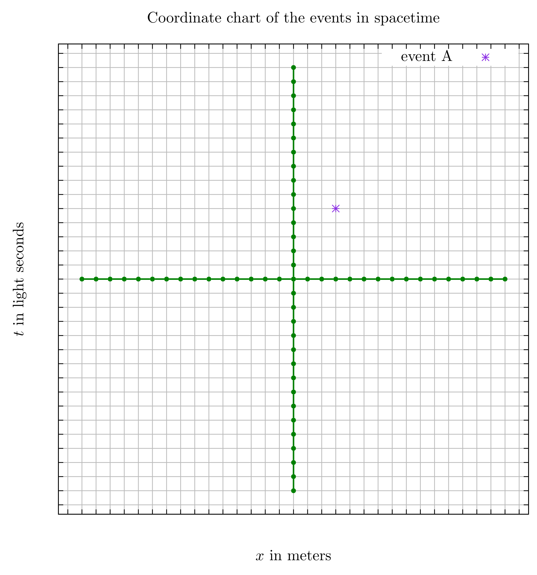
The German mathematician Hermann Minkowski utilized the property of coordinate charts (maps from manifold to  ) in making a useful geometrical tool called Minkowski graph. The idea is that on a graph paper we have two dimensions at our disposal. And, the Lorentz transformation shows that if relative velocity between two frames is along x-axis then the map of the coordinates
  and
and  to another coordinate system is identity. Therefore we consider the map from the events in the spacetime manifold to
  space (our graph paper) which includes only two coordinates
  and
and  as shown in the figure.

In this coordinate system (frame of reference), the event A has been assigned the coordinates (5,3). Also note that the time axis has been divided by the constant and, here, we define one light second as the time taken by light to travel one meter (or inverse of ).
Now each point in this graph (coordinate system) represents an event in the spacetime manifold. As the consequence, the evolution of a particle in the spacetime is mapped to a trajectory in the graph (which is drawn by the observer at the origin). This trajectory is called the “world line” of the particle. On carefully examining the transformations, one can note that when the relative speed between two frames is greater than the constant (which we now set to unity) then the factor  becomes imaginary. Furthermore, the factor approaches infinity when the relative speed approaches unity. In relativistic dynamics the total energy of a free massive particle is directly proportional to . Hence it would require infinite amount of energy to accelerate a particle near the speed of light.
The slope of the trajectory in the Minkowski graph is the inverse of the speed of particle with respect to the observer (who is drawing the graph). Therefore the slope of the trajectory is always greater than unity in the graph because a massive particle cannot be accelerated to the speed of light. A light ray always follows the trajectory of straight line with unity slope. The Lorentz transformation makes sure that the trajectory of the light remains same in all the graphs, corresponding to various coordinate systems.
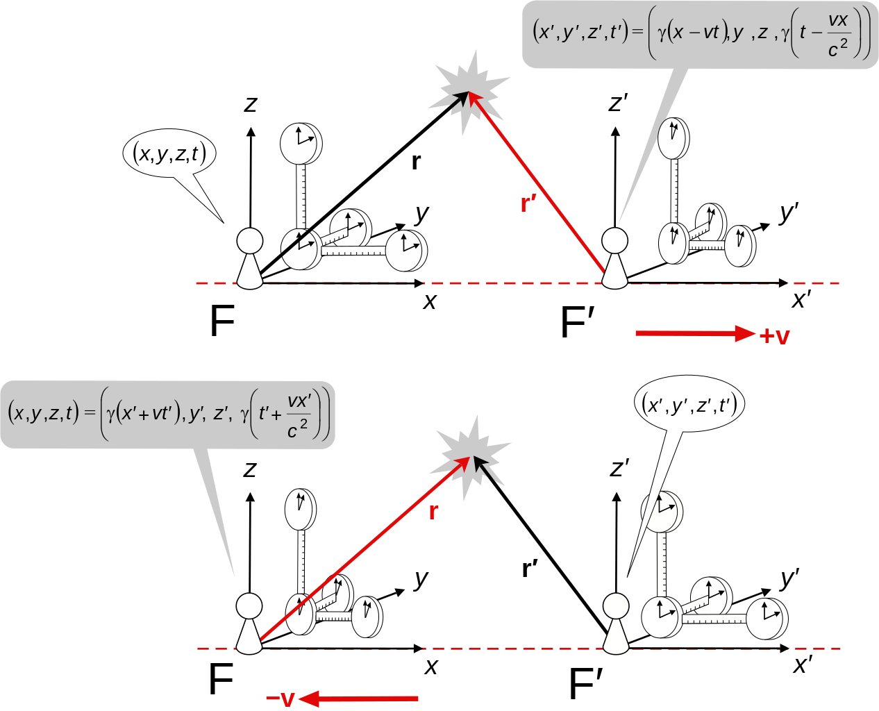
The Minkowski graph is quite helpful in comparing the physics from two frames. Consider two observers F and F’ moving with some relative speed.

Observer F uses her coordinate system to draw a Minkowski graph as shown in the figure above.
Now consider a massive particle at the origin with respect to the observer F’ (i.e  ) from time
  to
to  . So how will F draw the world line of the particle in her coordinate system (or Minkowski graph)? As you might have guessed, we will use the Lorentz transformation (because we have to map the information given in F’ to F). In other words we have to find the equation of the particle in coordinates of F subjected to the constraints
  and
and  in the coordinates of F’.
From the Lorentz transformation, the first constraint will give a trejectory equation  which F will interpret as the time axis of the observer F’ (because the line of constant x-coordinate giving t-axis and vice versa is a property of the orthogonal coordinate system in the space). Therefore F will draw a straight line in her graph with slope as inverse of the relative speed. Let
  meters per light second. The question now arises is that how will she mark the scale of that time axis in her coordinate system (or graph)? The second constraint gives a result that
  which means that a unit second in the coordinates of F’ is mapped t0 1.25 seconds in the coordinates of F. It means that the two events with a unit time separation at the origin in frame F’, are separated by 1.25 seconds in the frame F. Thus the graph of F will look like

The violet dots correspond to the events with unit time intervals and zero space displacements in F’ (hence it is the time axis for F’) while green dots in vertical line correspond to the events with unit time intervals and zero space displacements in F. Note that in the graph drawn by the observer F, the 15 units of her time is equal to the 12 units of the time in F’. It is consistent with the fact that  . This is why we say that moving clocks are slower.
Similarly, we can draw the x-axis of F’ in the coordinates of F using the same technique. Consider a situation in which  (simultaneous events) and
  . Using the Lorentz transformation and first constraint we get
  . This equation gives the x-axis of the observer F’ in the frame of F. Second constraint gives the relation
  . This means that a unit length (between two simultaneous events) in F’ is mapped to 1.25 meters in F. The graph now looks like
 The violet line with lesser slope represents all the simultaneous events of F’ (with ) in the coordinates of F where they are having different coordinate . Thus simultaneity is a relative concept and depends of the frame of reference.
In the end of this post, we will explain length contraction using the Minkowski graph. The length of a rigid rod is defined as the distance (in  space) between its end points at the same time coordinate (convince yourself!). Consider a rod of 2 meters length at rest in the frame F’. Let its first end point be at (4,
  ). Therefore, according to the definition of length, the coordinates of other end point will be (6, ). Now this rod will trace a “world sheet” in the Minkowski graph as shown in the figure below. The red dots on the lower violet line (the x-axis of F’) are the coordinates of the endpoints of the rod which are, according to F’, (4,0) and (6,0). They evolve in the time such that after unit second in F’, the coordinates are (4,1) and (6,1) (the couple of next red points on each red line) in F’. And it should be, because the 2 meter rod is at rest in F’.

Now how much length will the observer F measure? Let us say that at  light seconds she measures the length. Now according to the definition of the length, she will cut the world sheet of the rod with a line (to obtain simultaneous coordinates in her frame) and measure the distance between space coordinates. In this example the coordinates (pointed by the arrows) are 8 and 9.6. Thus the length of the rod is 1.6 meters in the frame F. This is called length contraction and this is why we say moving trains are shorter.
The main point to keep in mind are that in special relativity, an event in spacetime might not have same set of coordinates in different frames of reference. To map an event from one coordinate chart to another we must always use Lorentz transformation. If this is followed honestly, then all the paradoxes of special relativity can be resolved. One such paradox is “twin paradox” which I will explain in next post.
If you are wondering how I made these cool Minkowski graphs then head over here.


are tangent to the local lightcone everywhere.
is the corresponding luminosity distance.
are constant along each ray defined by the tangent vector
.


with the properties mentioned above


 with some constant relative velocity between them. There is an observer sitting outside the tunnel (observer A) and one sitting in the train (observer B). Now observer A will see the length of the train little shorter than the tunnel and observer B will see the length of tunnel little shorter than train (relativistic length contraction). Let the tunnel be a special one having two doors at the front (from which the train enters the tunnel) and at the end, capable of shutting down simultaneously. Observer A controls the doors. Now since the length of the train is smaller then that of tunnel according to A, she decides to shut down both the doors at that point of time when she sees the train completely inside the tunnel. On the other hand, the observer sitting in the train will deny the fact that the train can be captured by the tunnel as the train is longer than the tunnel according to her. But relativity says that the physics is invariant in any inertial frame therefore both the observers must concur on the facts (whether the train passes or gets captured).
 meters per light second with respect to Bob along x-axis, for some time (in the frame of the observer B) and then comes back to Bob with same the relative velocity. Now, naively, one can say that according to Bob, the time of Alice goes slower than him, hence when Alice returns, he must age more. According to Alice, Bob’s time goes slowly (moving clocks are slower for Alice too!) and therefore Alice should age more when she returns. But both Alice and Bob should agree on the same fact and here lies the paradox which everyone comes by when studying the relativity for the first time.
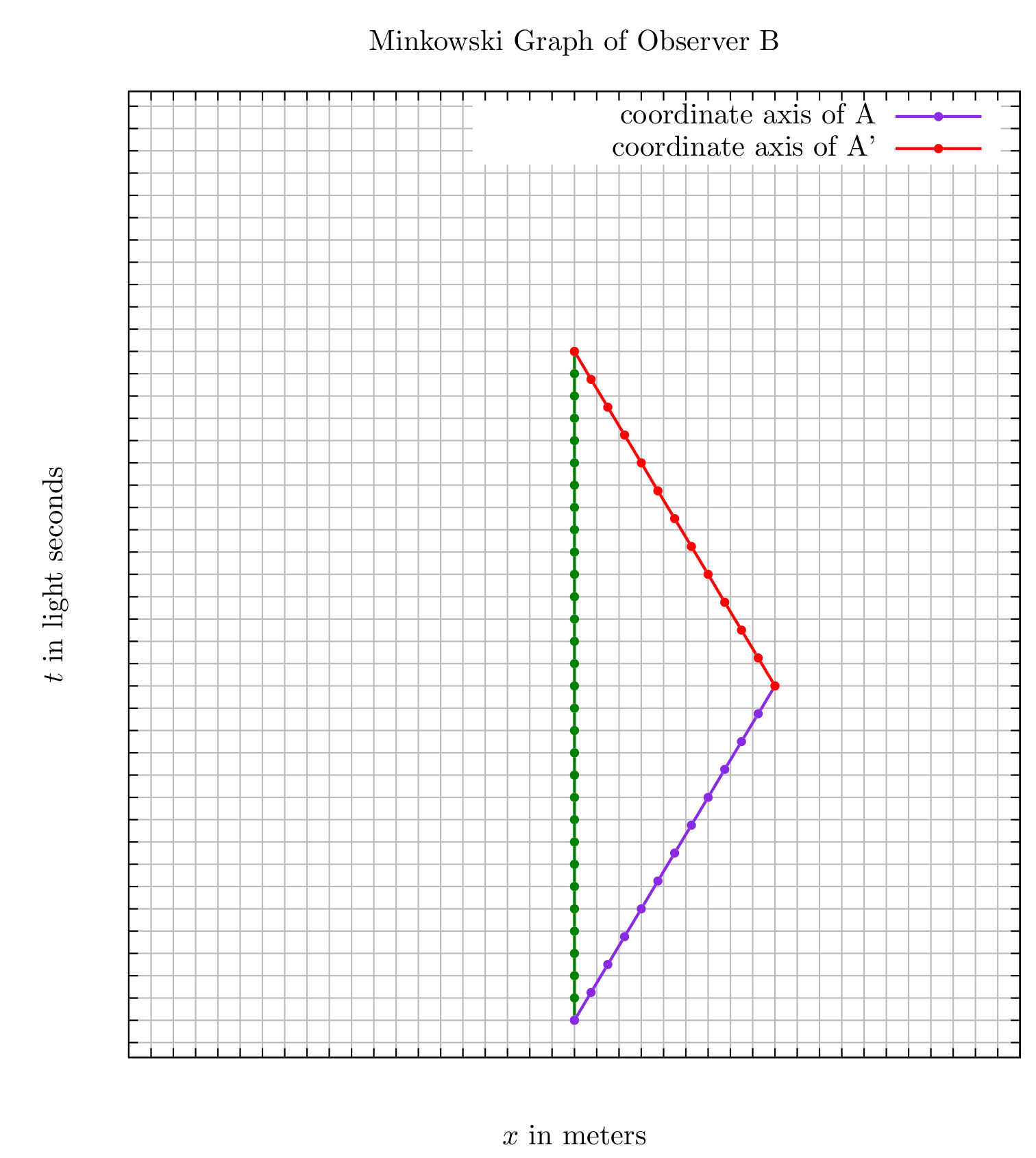


 and
and  , where
 and
and  ). The second postulate gives us a prescription to make scalars, in terms of what is known as metric. According to this prescription the squared path length is mapped to
  in a coordinate system constructed from
  . Here
  . Simple analysis shows that it must have the dimension of
  . In another coordinate system with the coordinates
  and
and  the squared path length is mapped to
  . Note the same constant
  . This is the starting point of the derivation of the Lorentz transformation in the standard relativity textbooks (although they arrive at this expression using light rays which is misleading sometimes). The Lorentz transformation is a relation between the coordinate systems of two inertial observers, assigned to the same events in the spacetime manifold
  meters per second which is the speed of light. The derivation of these transformations can be found in any standard textbook on relativity or in Wikipedia (
 and
and  belonging to Euclidean space. I will give you the distance between them by computing
  .
. and
and  and define a
  matrix
 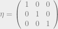 . The distance between two points can now be given by
  (here ‘.’ represents matrix multiplication). Note that the definition of distance depends on the matrix
  . Physicists and mathematicians call
  where
where  .
.