C++ programming language, just like a regular English language, has concept of “genericity”. For instance, the word “bank“, in English, is generic in the sense that the word can mean an institution (noun) or an activity (verb). The meaning is inferred from the context of the word usage.
Genericity introduces certain degree of flexibility in the language. The flexibility covers etymologically related or even, in some cases, unrelated meanings (or links?). For instance, “bank” may refer to financial institution as a noun or, related activity as a verb, or edge of a river as an unrelated (to the institution) noun. Basically, genericity can be viewed as minimizing the vocabulary and maximizing the utility or means to control the complexity of a language.
Similarly, in C++ language, there is a notion of generic programming which is implemented by using templates. Consider the following C++ code
template<typename T>
void Exchange(T& a, T& b)
{
T temp = a;
a = b;
b = temp;
}
This function, Exchange, can be used for floats or ints alike to exchange the value like so
int a = 10;
int b = 20;
float c = 100;
float d = 200;
Exchange(a, b); // a becomes 20 and b becomes 10
Exchange(c, d); // c becomes 200 and d becomes 100
Note how the function Exchange is used for both ints and floats type. Based on the context, int and float calls, compiler generates two copies of Exchange function, one each for int and float type respectively, using which the values of variables are exchanged.
I am sure there must be a mnemonic-al way to Unreal’s collision configuration, independent from C++ or blueprint. Maybe Stephen’s explanation can demystify parts of the collision. In this blog-post I shall attempt to create an appropriate mnemonic device using abstraction(s).
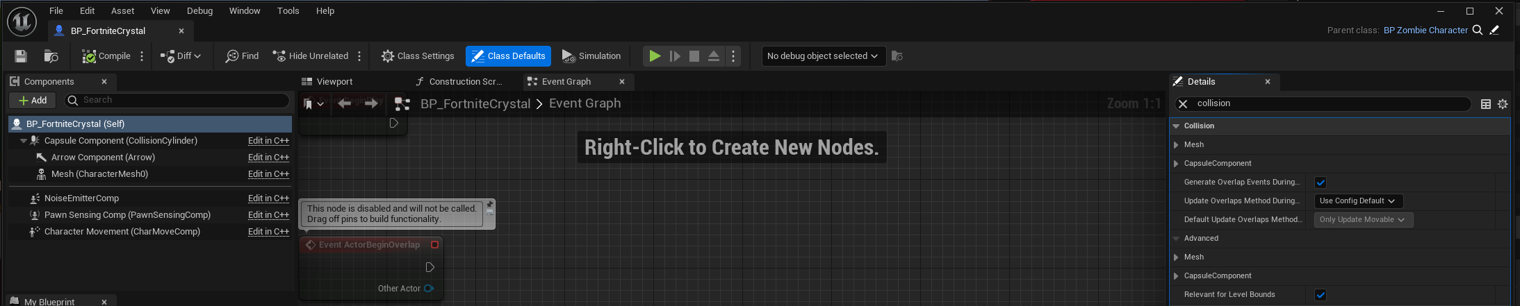
In Unreal, UPrimitiveComponent is the scene component class with collision specific data and render-able geometry. Any specific object, that you see placed or spawned in the level, having certain shape, probably has a scene component derived from UPrimitiveComponent. The collision settings are configured in the details panel of the appropriate blueprint
The picture above shows collision configurable for capsule component. Similarly there is one set of configurables for Mesh component. Rest of the components have no such collision configurable.
To get an overview of all the collision configurables, one can click on the parent of Capsule Component (BP_FortniteCrystal here) to get the following in Details panel
We note that collision configurables for both the mesh and capsule component are shown which pretty much sums up the collision configurable for the blueprint.
Next, we have the following configurables
Simulation Generates Hit Events
Generate Overlap Events
Can Character Step Up On
Collision Presets
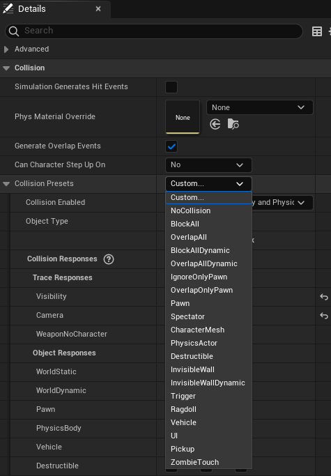
Not sure what point 1 does. Point 2 makes sure that the component is involved in generating overlap events. If you want the ability for a character (a pawn with ability to walk) to step on, check point 3. Finally we come to Collision Presets
The picture above shows some default collision presets (except ZombieTouch and Ragdoll presets which are custom presets, which I may explain later). You may select the preset that best fits the component. For instance in C++ code we have the following equivalent
Mesh3P->SetCollisionProfileName(TEXT("Ragdoll"));// Go to Project Settings -> Collision -> Preset -> Ragdoll
}
...
}
The SetCollisionProfileName selects the Collision Preset, when using C++, during runtime, when zombie character is killed and becomes a mere ragdoll.
The idea is that each Collision Preset (or profile) makes the component sensitive to raycast or spherecasts or some sort of cast (by a channel), sent from external source, appropriately (corresponding to trace).
Channels decide the nature of sensitivity, in a sense, to the trace being done. For instance, in the picture of collision presets below, there are three categories, one custom (WeaponNoCharacter) and two default (Visibility and Camera). BTW, here is Epic’s blog-post on the subject. Also objects can decide the nature of sensitivity to the trace being done.
Traces offer a method for reaching out to your levels and getting feedback on what is present along a line segment, LineTraceMultiByChannel, or sphere tube and all that (SweepTestByChannel).
Consider the following custom collision presets
for, say, skeletal mesh component. This implies that the component registers blocking hit only for WeaponNoCharacter channel trace and ignores Visibility and Camera channel traces.
Similarly the component is sensitive only to the objects of WorldStatic, WorldDynamic, PhysicsBody, and Destructibles category.
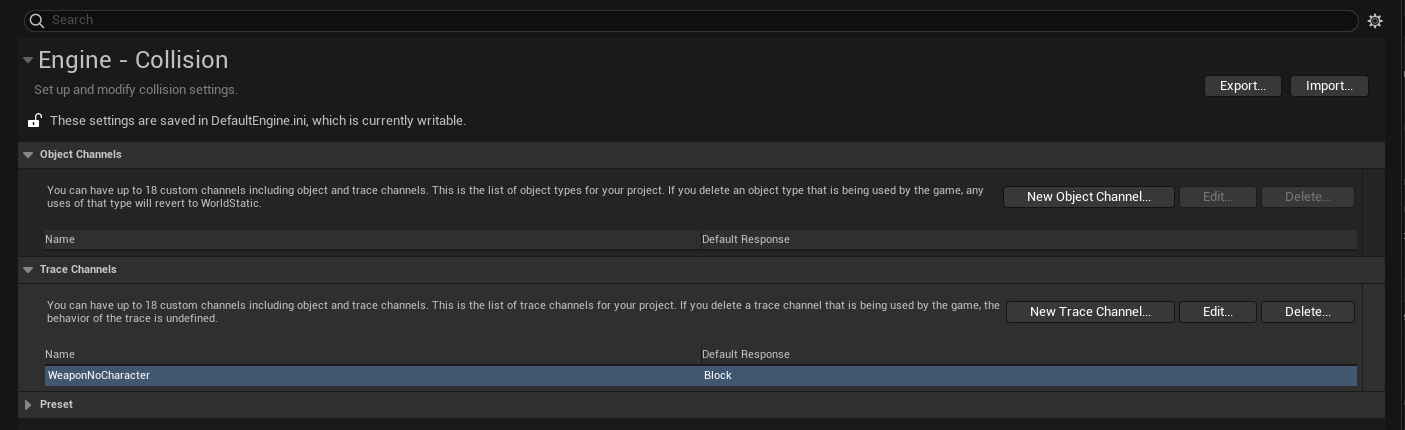
A custom trace channel is created in Project Settings
and to use in C++, open Config/DefaultEngine.ini and look for the channel name (here WeaponNoCharacter). You may find something like
SOLID principles for object oriented programming are demonstrated in action here. Whilst coding my FPS game, I observed couple of violations (SO) the second time I modified a section of code. This is the classic example of how context helps in catching such violations. Consider the following hierarchical class arrangement
class SUNOVATECHZOMBIEKILL_API ASTPickupInventory : public ASTPickup{
public:
    virtual void GiveTo(Pawn* Target) override;
...
}
class SUNOVATECHZOMBIEKILL_API ASTPickupWeapon : public ASTPickupInventory
{
...
}
and finally implementation of GiveTo() function like so
void ASTPickupInventory::GiveTo(Pawn* Target)
{
	if(Target == nullptr)
	{
		return;
	}

	Super::GiveTo(Target);

	ASTInventory* Existing = Target->FindInventoryType(InventoryType, true);

	if (Existing == nullptr)
	{
		ASTInventory* Inv = nullptr;

		// Spawn the inventory type class object and attach to pawn
		UWorld* const World = GetWorld();
		if (World != nullptr)
		{
			...
		}
		else
		{
			UE_LOG(LogSunovatechZombieKill, Log, TEXT("No world found, can't spawn actor of class %s"), *InventoryType->GetName());
		}

		// Add inventory to target and equip
		if(Target->SwitchToRecentPickup())
		{
			Target->AddInventory(Inv, true);
		}
		else // or not
		{
			Target->AddInventory(Inv, false);
		}

                // This looks out of place
		ASTWeapon* MyWeapon = Cast<ASTWeapon>(Inv);

		// Generate circular doubly linked list for switching weapons by rotation
		if(MyWeapon)
		{
			Target->GenerateWeaponCDL();
		}
	}
	else // ok this pickup already exists in inventory
	{
                // This looks out of place as well
		// if weapon, increase the ammo
		ASTWeapon* MyWeapon = Cast<ASTWeapon>(Existing);

		if(MyWeapon)
		{
			MyWeapon->AddAmmo(10); // to do: move this code to STPickupWeapon maybe
		}
	}
}
The “out of place” code may require data member (or member function) of ASTPickupWeapon class, for instance AddAmmo() may require amount belonging to the class.
The SRP (Single Responsibility Principle) says that class should have only one function, here, involving general inventory only. Specializing to ASTWeapon seems responsibility of ASTPickupWeapon. Open/Close principle says that class should be open for extension and closed for modification which also seems like a violation here. This implies violation when weapon specific modifications are applied. Hence if SRP is violated, so is Open/Close principle.
A simple solution is to write overridable methods like so
class SUNOVATECHZOMBIEKILL_API ASTPickupInventory : public ASTPickup{
protected:
	/**
	 * @brief Function for dealing with non-existant and post inventory spawn procedures
	 */
	virtual void DealWithNonExistentInventory(ASTInventory* NonExistingInventory, Pawn* Target);

	/**
	 * @brief Function for dealing with existing inventory procedure
	 */
	virtual void DealWithExistingInventory(ASTInventory* ExistingInventory, Pawn* Target);
...
}
by doing this, we have opened passage way for child class ASTPickupWeapon to do ASTWeapon specific computing.
void ASTPickupInventory::GiveTo(Pawn* Target)
{
	if(Target == nullptr)
	{
		return;
	}

	Super::GiveTo(Target);

	ASTInventory* Existing = Target->FindInventoryType(InventoryType, true);

	if (Existing == nullptr)
	{
		ASTInventory* Inv = nullptr;

		// Spawn the inventory type class object and attach to pawn
		UWorld* const World = GetWorld();
		if (World != nullptr)
		{
			...
		}
		else
		{
			UE_LOG(LogSunovatechZombieKill, Log, TEXT("No world found, can't spawn actor of class %s"), *InventoryType->GetName());
		}

		// Add inventory to target and equip
		if(Target->SwitchToRecentPickup())
		{
			Target->AddInventory(Inv, true);
		}
		else // or not
		{
			Target->AddInventory(Inv, false);
		}

                DealWithNonExistentInventory(Inv, Target);
	}
	else // ok this pickup already exists in inventory
	{
               DealWithExistingInventory(Existing, nullptr);
	}
}
Recently, whilst making an FPS game, I happen to implement a feature involving blood. The idea is, when you butcher zombies, their post-coagulated(?) blood spills on the floor they are standing or rather creeping on. Clearly we need to use something “other than” UParticleSystem for the purpose because we are not looking those particle effects which look like spray in air
The gif shows two kinds of blood effects. One is the blood-sprayed-in-air effect (particle effect) and other is splat on ground (decal).
For particle system we have the following Unreal C++ declaration
You may wonder why such philosophical title appeared in the blog having a playful physics theme. The idea here is to elicit a bug (or a feature in my sister’s thinking) in being which everyone knows yet so few admit.
The bug is the inability to appreciate. From personal experience, when I was a high schooler there used to be a buzz about being IITian. We were told that an IITian bags more respect than Bill Gates, perhaps, in the context of software engineering. That used to supply a push (both mechanical and mental), to excel in current study. The practice that went to prepare IIT’s entrance examination coupled with the IIT alumnus’s achievement would stand like a testament to the reputation that we realized second (so on) hand.
Then I cleared the entrance and got selected to pursue my undergraduate studies at IIT Roorkee. And to my surprise, I met bit of people who didn’t take any, not some, any, pride being IITian. This anti-fascination-ism reached to the point that someone (a non IITian) asked me “What have you done being an IITian” with possible intention of comparing with non-IITians. This is something I would not have said even if I had not cleared the IIT-JEE.
Similar is the case with Earth’s pollution. If you really want to understand the context, try computing the ratio of number of planets discovered by Mankind to number of planets with conscious beings, something even a ten year old can imagine and visualize. Given such extreme figure, how can one even think of polluting the environment deliberately, for instance by maintaining the space race. The problem is same, inability to appreciate.
Lastly, since this is playful physics blog, I’d like to mention multiplatforming. Those who have taken into account the definition of Turing Machine, may understand how satisfying it is to play a game (run a same program) on desktop, laptop, mobile, and so called next-gen platforms. Fun is in the ability to play on internet with players from different platforms, called cross-play. Achieving is certainly not hard, Namco has so aptly demonstrated, and also not pretty obvious, 2K team has so aptly demonstrated (mild sarcasm). Yet you may find “them” (players?) complaining and not appreciating the feat Namco has achieved. What is like achieving a miracle for 2K (sic) is seemingly not worth consideration for Namco’s player(?) base.