So it has been more than a week since I wrote my last blog post. Although, time to time, I was tempted to write the sequel, but I had to distance myself from that temptation. I have been studying David Griffiths’s “Introduction to Elementary Particles” and much of my time has been devoted to it. Hopefully one day I will know Particle Physics well enough to blog about it.

So by now I am sure you know what it means when we say something is linear. This is the beginning of linear algebra. It is a very beautifully constructed algebra which physicists use in their daily life (like in Quantum Mechanics, Special theory of Relativity and Classical Mechanics). I don’t intend to start off with the abstract Hilbert Spaces (basically a set of linear vectors with some axioms) and define linear maps, inner product structure and so on. Instead I will try to demonstrate the linear algebra “at work (using Quantum Mechanics)” without worrying too much about mathematical vigour. Now I must warn you  that this mathematical vigour is absolutely necessary to not only appreciate the beauty of mathematics (I am a big fan of the water-tight derivations done by the mathematicians!) but to get a better understanding of Quantum Mechanics (least you land up in the situation where it might seem that Quantum Mechanics is inconsistent with itself). Basically in the following demonstration, I will define certain mathematical quantities in a very loose way (loose enough to drive any mathematician, with slightest respect for mathematics, crazy) and mix them with the postulates of Quantum Mechanics without explicitly stating them. For instance, the example I gave in last post, deals with the linear vectors belonging to a linear vector space equipped with inner product structure (or Hilbert Space). I believe that this way I wont make the subject abstract enough for the people new to Linear Algebra and Quantum Mechanics.

So Quantum Mechanics says that the physical states are linear. This might not surprise you and you might think that it is obvious (maybe after going through the example I gave in last post). But think again! This statement is powerful enough to lead to certain results which you might not consider obvious.

Before going further I want you to see this video and try to understand the problem it states in the end.

At first it might seem too confusing. But we will go, step by step, and try to reproduce the experimental results using Quantum Mechanics. I am considering the case when only one electron is shot out at a time from source . I associate a linear state vector to represent the electron at source. Now the states representing slit 1 and 2 be and respectively. The screen is basically a real number-line where each point represents a state written as . Note that is a continuous parameter here.

Now recall last post in which I gave an example of “creating” a set of persons “using” two persons (basis). In general a person can be written as where the  will tell me the resemblance of person C with person A or B. Now I define a term inner product as a function (a linear map) which maps the ordered pair of linear vectors into a scalar complex number. This complex number gives the component of the linear vector on other linear vector ( will give resemblance).

Consider the inner product of person A and B written as . Now we know that they don’t resemble at all. Hence should be equal to (state B has no component on state A whatsoever). The states and are said to be orthogonal. Also we know that state completely resembles with itself and so does state . Thus (I can assign any number to this inner product). I have normalised the state vectors and (because the number I assigned is ). They are now called orthonormal linear vectors.

To find the component of along , I just need to evaluate the inner product . So

and

The resemblance of state C with state A is and with state B is . This is the idea of inner product.

In Quantum Mechanics it is used in a different way. We have state C (now representing a physical state and not a person) given in terms of state A and state B (again physical states). Now if a system is described by state then is the amplitude of state to exist in state (read it this way and understand it this way!). is the probability with which we will find a system described by state in state . The probability of state C to exist in state B is . So instead of resemblance, the component of vector gives an idea about the probability. This is the basic rule which the nature seems to follow. Max Born was the guy who realised this.

The question which might arise here is that before measuring the system it was in state . Mathematically it is called superposition of states and . But what is it physically? Does it mean that if a system is represented by state then it is existing in both the states and , simultaneously? Quantum Mechanics gives no answer to this. It is something that you have to interpret yourself.

Although you might try to relate it to the example I gave in previous blog post, but you must understand that these physical states are very different from the states representing the persons in the sense that there are no “extra variables” (like lefty, hindi and lazy) which make up the states. These states are fundamental and nothing is implicit. For instance state represents slit in double slit experiment and that is it. So from now on, the physical states are to be considered without any extra variables.

Now I define another linear entity “operator”. It is again a linear map (or function) which maps a linear vector into another linear vector. Operator is denoted by a letter with a hat . So the operation of a linear operator on a linear vector is defined as , where is a complex number. Now I can represent same operator by . This is known as “outer product notation”. Let’s check weather this notation is compatible with the definition of operator.

Here . State might not be normalised.

In Quantum Mechanics all kind of actions on a state vector are represented by linear operator. There are operators corresponding to time translation, space translation, space rotations and observables. By definition theses operators map a linear vector (physical state) to another linear vector (another physical state).

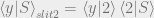
Suppose you are standing on the other side of slit (opposite to electron source). Further suppose that slit is closed. Now what state would you assign to the electrons coming out towards you? Now the slit will act like a source. You will say that the state of electron is . Thus the state has been mapped to state . This is the handiwork of slit and thus we should associate an operator with it. How should the operator look like? Operator should be able to tell us the amplitude of state to exist in state . Consider the form . Now . This operator maps the state to state and also provides the required amplitude. So good! Similarly, on closing slit , we will find that the operator corresponding to slit is . In hat notation, I assign operators and to slit and respectively.

Now we have necessary tools to work out the Quantum Mechanics of this experiment. The states for double slit experiment we have are and and the operators are and . Now if I shoot one electron after other, then (assuming no absorption by the slit wall) I should be able to get corresponding detection at certain state (on the screen). So one electron is emitted out from source and we detect one electron on screen. I should evaluate the amplitude of state to exist in state or the number . Then I can get the probability with which an electron will be detected at by evaluating .

We saw that the slits have the ability to map state to state or state and these are the only two alternatives. This should make us conclude that state is made up of state and with certain amplitude (which is nothing but probability for state S to exist in slit 1 or 2) for each of them in a linear way. Thus

and

with little re-arrangement

Feynman’s way

In Feynman’s lectures volume III, he obtains the last equation in a very beautiful and intuitive way. He first states two rules

when an event can occur in several alternative ways, the probability amplitude of the event is the sum of  amplitudes of each alternative way considered separately (provided experiment is not capable of determining which alternative is actually taken). If the experiment is capable of determining, then the probabilities should be added.

and

if  a particle goes through a route then the amplitude for that route can be written as a product of amplitude to go part way and amplitude to go rest of the way.

In our double slit, the particle can reach state by two ways (which can not be distinguish just by detecting the electron at the screen) thus the amplitudes must add

The experiment is going via superposition of two possible alternatives. Now using second rule we can say that (I have changed the order since it is better to read from right to left). Similarly and we end up with the same equation.

Now is a complex number and so is , but is a continuous variable which can take any value like and so on and for every we should have corresponding amplitude. It is better to represent by a function say . Same goes for . Thus

.

You can put and inside the functions. It won’t be a problem becase they are constant.

The probability to detect a particle on screen (at certain y) is . So now you see why we get interference pattern? The probability contains a cross term which precisely shows interference.

You see, how by associating linear vectors to physical systems (and using some additional assumptions) we found an astonishing result of interference. If you want you can watch the video again (keeping this treatment in mind). Now I am going to discuss the physical implications of this treatment.

First you might be wondering about the nature of electron. Is it particle? Or is it a wave? Well it is neither. Wave and particle are classical concepts which are often mixed with the name “wave particle duality” to describe quantum entities. I consider it as misleading specially for new people learning Quantum mechanics. You see in Quantum Mechanics we just say that it is a linear vector by which we mean that it is an entity that is linear in nature. There is absolutely no need to draw a picture of the electron in your mind (like a rigid ball or wavy curve or mixture of both).

Now since it is a linear vector it can exist in superposition of various states. So it is not necessary to imagine an electron going through a particular slit (when you are not observing the electrons at the slit). It is going through both the slits (if this is what you want to hear). And in Quantum Mechanics you will come across such examples many times.

In the video you have seen that interference pattern disappears when one tries to observe the slits through which electron goes. So the act of measurement destroys interference pattern. Of course we can show that using Quantum Mechanics, but it involves concept of Tensor Product or Direct Product of linear vectors, which is out of the scope of this article. Feynman, on the other hand shows (by following those two rules) how the measurement destroys interference without “explicitly” talking in terms of direct product. I dont want to repeat it, so I recommend Feynman Lectures Vol III chapter 3.