This post may be considered a continuation of the post Addressing The Addresses or a separate read. We are basically interested in understanding how type-casts are done at assembly level, corresponding to C++ language, which may give a clue about the address arithmetic being performed leading to the offsets discussed in the post I mentioned in the beginning.
First let me demonstrate the typecasting of primitive types (I am taking some stuff from this wiki page). Consider the C++ code
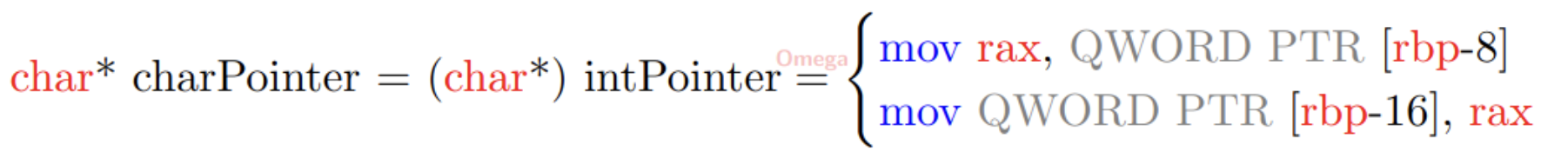
In the last line we are doing an explicit type conversion from int to char.
From assembly instruction perspective, there is no difference between int and char as far as the casting is concerned. Information about one pointer (of type int) is shared with the different pointer (of type char). Only the dereferencing bit differs like so
char b = *aP;         mov     rax, QWORD PTR [rbp-8]
                      movzx   eax, BYTE PTR [rax]
                      mov     BYTE PTR [rbp-9], al
while for int
int d = *cP;          mov     rax, QWORD PTR [rbp-24]
                      mov     eax, DWORD PTR [rax]
                      mov     DWORD PTR [rbp-28], eax
for char type of dereferencing, BYTE is read, while, for int type of dereferencing, DWORD is read.
Moving on, we now consider user defined data types, specially classes. Consider the following code
#include <iostream>
class UObjectBase
{
    int a;
    int b;
};

class UObject : public UObjectBase
{
public:
    virtual ~UObject() = default;
};

// Type your code here, or load an example.
int main()
{
    UObjectBase bar;
    UObjectBase* ptr = &bar;

    UObject* fp = (UObject*) ptr;

    std::cout << &bar << '\n';
    std::cout << fp << '\n';
}
The out put of above program may be
0x7ffe4dd2f998
0x7ffe4dd2f990 // 8 bytes offset
however on removing the virtual function (the destructor ~UObject()) may lead to the out put
0x7ffe4dd2f998
0x7ffe4dd2f998 // same address
Here, we are basically down casting from UObjectBase to UObject and that leads to the offset of 8 bytes in presence of virtual function (vtable). The assembly code instructions (generated vis godbolt) look like
In presence of the virtual function (or vtable) there is an instruction to subtract 8 bits from rax which creates the offset in addresses shown in the out put. This example was taken from stackoverflow post.
In the book “Effective C++, third edition”, item 27, Scott Myers points that
… a single object (e.g., an object of type Derived) might have more than one address (e.g., its address when pointed to by a Base* pointer and its address when pointed to by a Derived* pointer). That can’t happen in C. It can’t happen in Java. It can’t happen in C#. It does happen in C++.
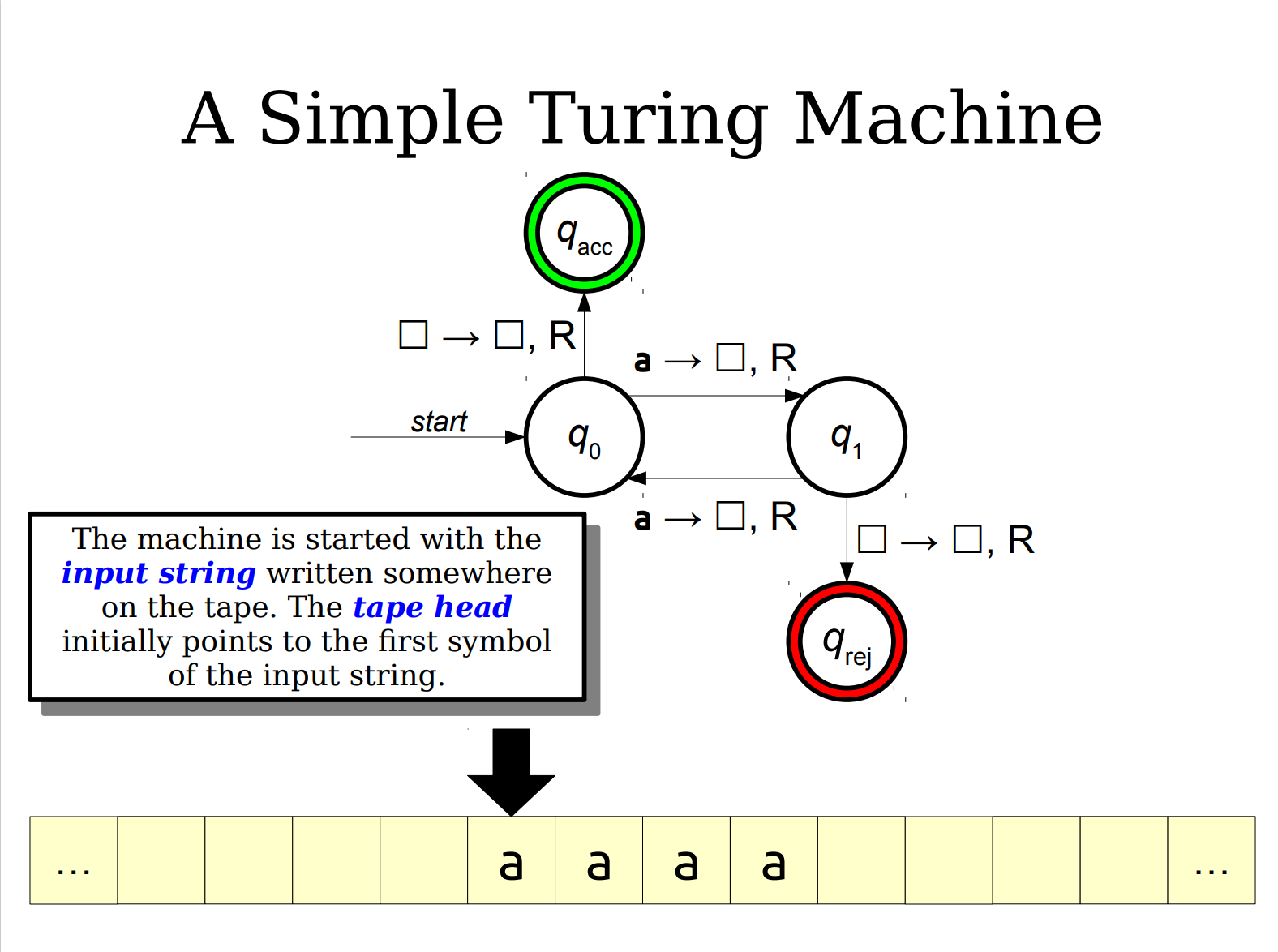
In my books, computers are the best machines humans have ever built. A big wave to Alan Turing, you are the thinker I may resent if at all (well Paul Dirac and Darwin are in the same league). All Turing machines (i.e computers) have tape to read from and to write to, like so
The purpose of this blog-post is to understand the implications of “how” the tape is read. Based on this notion of “how” variety of “meanings” (software data-types) emerge if considered at low enough level of abstraction (assembly language).
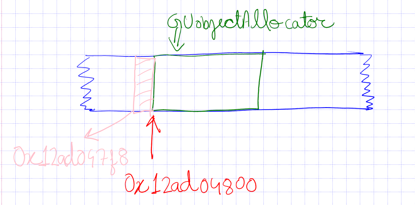
We will take a live example from Karma, where we have a UObject pool allocator. The idea is to allocate a block of memory for UObject, for instance, AActor spawn (which is done in the routine SpawnActor()). Another example is UClass (which is great grand child class of UObject). Our pool allocator, GUObjectAllocator, allocates the space from the blue strip, representing Karma’s pre-allocated memory, and returns the address in red, meaning the subsequent block of memory addresses, determined by the size of UClass, have been reserved.
However, the following error message (pardon the Normal block address which is not specific to the example I have in mind, written above) started appearing on application close (or, to be precise, on freeing the blue block of memory at application close)
Thus began my search for the grand resolution of the issue. I posted the error message in CppIndia Discord Server. In the response, I was suggested to use Address Sanitizer (ASAN) to look out for the cause of such issue. And sure enough, Xcode ASAN greeted me with the following
==36231==ERROR: AddressSanitizer: heap-buffer-overflow on address 0x00012ad047f8 at pc 0x00010084d208 bp 0x00016fdfcc20 sp 0x00016fdfc3e0
WRITE of size 64 at 0x00012ad047f8 thread T0
    #0 0x10084d204 in __asan_memset+0x104 (libclang_rt.asan_osx_dynamic.dylib:arm64e+0x41204) (BuildId: f0a7ac5c49bc3abc851181b6f92b308a32000000200000000100000000000b00)
    #1 0x102a971d4 in Karma::FGenericPlatformMemory::Memzero(void*, unsigned long) GenericPlatformMemory.h:72
    #2 Callstack .....

0x00012ad047f8 is located 8 bytes to the left of 1280000-byte region [0x00012ad04800,0x00012ae3d000)
allocated by thread T0 here:
    #0 0x10084ee68 in wrap_malloc+0x94 (libclang_rt.asan_osx_dynamic.dylib:arm64e+0x42e68) (BuildId: f0a7ac5c49bc3abc851181b6f92b308a32000000200000000100000000000b00)
    #1 0x102aa5b08 in Karma::FMemory::SystemMalloc(unsigned long) KarmaMemory.h:124
    #2 0x102aa5a24 in Karma::KarmaSmriti::StartUp() KarmaSmriti.cpp:25
    #3 0x1029ab45c in Karma::Application::PrepareMemorySoftBed() Application.cpp:65
    #4 0x1029aade8 in Karma::Application::PrepareApplicationForRun() Application.cpp:54
    #5 0x10000772c in main EntryPoint.h:79
    #6 0x195923f24  (<unknown module>)

Some report on Heap Overflow
==36231==ABORTING
I have put bold font to the text of interest. The FGenericPlatformMemory::MemZero() is doing the “illegal” writing to the block of memory at address 0x00012ad047f8 which was not the address, 0x00012ad04800, returned by GUobjectAllocator. Furthermore this fact is reinforced by the message “0x00012ad047f8 is located 8 bytes to the left of 1280000-byte region [0x00012ad04800,0x00012ae3d000)”. So who or rather how is this offset of 8 bytes is being introduced?
The typecasting done while generating the UClass object, here
is the reason for the offset of 8 bytes leading to the error message because of writing in the place that is not supposed to be written by the app. I have marked the “illegal” block of memory with pink in the cartoon above. The rectification is simple enough
The reinterpret_cast basically type casts the data type without introducing offsets in the address. Thus the conversion from UObjectBase* to UClass* is achieved with ReturnClass having the address value of 0x00012ad04800, which is the legal block of memory reserved by Karma’s pool allocator.
This might raise a question on the comparative working of reinterpret_cast and C-style cast that we leave to the future. A thing that can be said is for that we will be needing assembly language equivalent of the code, something along the lines of this article.
I believe a good game-dev environment should be capable of supporting all-platform philosophy and this can be achieved by being open enough to strive for enough learning and compassion.
The purpose of this blog-post series is to explore and show just that. We begin with the study of a cross-platform real-time graphics driver.
Vulkan is a cross-platform 3D graphics API and graphics driver meant for Real Time rendering. The best feature, for me personally, is the degree of control provided with the fortune of low-level programming tools which clears up the graphics rendering pipeline concept for enthusiasts and delivers major lesson for the uninitiated (who survive at the convenience of easy GL type function calls, not to say I’m not Glad, pun intended). Our friend Cherno is a great propagator of the API who introduced me to Vulkan. But we gonna extend his legacy and put the concept of cross-platform to test with all the stress-tests known to tech-kind.
Along with the official tutorial I have consulted Travis Vroman’s videos and some off-mainstream videos. In context of Karma, we don’t need to hook Vulkan as sole beneficiary but rather as any other regular library with enough fluidity of switching like so
Here we see it is matter of single line to change the rendering API for Karma. Clearly I plan to implement Metal/DirectX in future. Remember we need a decoupled way of hooking the library for cross-platform reasons. This results in the following folder hierarchy generating enough basis for the abstraction we are striving for
The entities thus formed are equipped with the ability to hook with high specificity and moral values (minding own business and not interfering with others in any sense). Then it becomes my job to deal with the decisions, for instance, how much ground to cover with how much depth such as to maintain the overall harmony in Karma. At this point in time, the following flow-chart captures the essence of Karma
Clearly, Vulkan is part of Rendering Engine, which, is an abstraction that can be visualized as a magical (not mystic though) box with the following diagram
The layer takes care of what platform we are running on and which rendering API we are rocking with. Then the concept of cross matching (within the scope of API-Platform support alliances) is obvious. Let me outline of the Rendering Engine (RE) functioning. In a typical Rendering loop, the following lines of code are a must
virtual void OnUpdate(float deltaTime) override
{
    Karma::RenderCommand::SetClearColor(/* Some Color */);

        Karma::RenderCommand::Clear();

    Karma::Renderer::BeginScene();

    /* Process materials and Bind Vertex Array. */

    Karma::Renderer::Submit(/* Some Vertex Array */);

    Karma::Renderer::EndScene();
}
Now we would want our APIs (Vulkan/OpenGL or whatever) to conform to these simple static function calls. That is where the RE magic comes in. No matter what the working philosophy of graphics API is, we need to channel that into a working set of routines such that the above OnUpdate function, called in the game loop, which can be identified with Karma's Rendering Handle in the flow chart, makes sense (works). Let me define and explain the actors of this play
Vertex Array: Can be imagined synonymous to a well behaved container of Mesh and Material (defined here). Each API should have its corresponding instantiation of Vertex Array.
Render Command: Is a static class with the rendering structure (curtsey TheCherno) and with the runtime-polymorphism responsibility to direct the calls to appropriate API (specified here). It holds the reference to RendererAPI which could be Vulkan or OpenGL after doing their initialisation specified in RendererAPI.cpp.
Renderer: A data-oriented static class containing the scene information (for instance camera) for relevant processing, and, rendering API information for Karma.
There is an entire branch in which we attempt to hook Vulkan API and which succeeded almost as expected (with some reservations and I plan to do a stress test with large number (millions perhaps billions of triangles)). But let me first chalk out the partial-abstractions acting like an interface between the static routines, in the above block, and low level Vulkan commands. The following are the Vulkan adaptations of Karma’s abstract classes.
Please note I am using the video as raw material and vulkan-tutorial for regular checks in what I understand and write henceforth.
The goal for any decent graphics API is to provide means (tangible and intangible) to map the coordinates of a triangle (read my blog-post for underlining importance of triangles in Real Time rendering) to the pixels on monitor or screen. This is it! What basically creates the market for various APIs IS the need for a hardware friendly algorithm which is considerate enough not only for scaling to billion triangles but also for providing natural fit to the taste of the programmer. Taste may include various levels of legitimate control based on what the programmer may think serves the purpose.
Playing video games is not only fun but also an engaging activity which can lead to catharsis. But there is a novel dimension to this activity which many players enjoy even more. It is building the game itself. This is the reason why many games come with level editors. For me, video games are not only the mode of experiencing a given world, but also an opportunity to modify and enhance that world to express myself.
I find game programming intellectually satisfying. It basically translates to building an interactive world and providing a structure to that world by enforcing the rules set by the programmer, who, then, can witness the world evolve under those conditions. It is an ecstatic activity to watch your own creation unfold before your eyes which you experience as being an integral part of.
Almost all the games are made using Game Engines. Unreal Engine and Unity are the prime examples of open-source game engines available in the market. As a serious game developer, it is a good exercise to write your own game engine. It not only exposes you to the current state-of-the-art game development methodologies but also provides the complete control over the scheme of building process. With this in mind, I have embarked upon the journey of writing a game engine myself. I call it Karma and it can be found here.
A game engine has several sub-systems including a rendering engine. As the name suggests, its aim is to draw (render) graphics corresponding to the visible game objects (like player character, weapons, mountains etc), on the screen. The engine has to draw the entire scene quickly enough (typically one frame is rendered within 16.6 milliseconds) so that 60 frames can be drawn in one second and illusion of continuous motion (of game objects) can be generated in real time. In this blog-post we will be focusing on rendering graphics.
Computer graphics in real time are rendered using triangles. They are the building blocks of CG just like strings are the building blocks of matter in String Theory (or, for faint hearted, cells are the building blocks of life in biology). Triangles are optimal candidates for real time rendering because
triangle is the simplest polygon
triangle is always planar
triangle remains triangle under most transformations
virtually all the commercial graphics-acceleration hardware is designed for triangle rasterisation
A simple demonstration of triangles generating graphics can be found here and here. Therefore rendering a triangle in an efficient manner is a crucial step in real time computer graphics. I will demonstrate here how Karma does it.
First grab the code from my GitHub repository. GitHub is a service which provides software hosting (for free!) and version control using Git. One can track down the software in its various stages of development back in time. Make sure you have Git installed. Open the cmd (on Windows) or shell (Linux) and type
The above lines of code basically download the Karma engine and reset the state of the local repository to the state, back in time, when first triangle was rendered by the Karma. Now depending of the platform proceed as follows
Windows
Make sure you have Visual Studio 2017 (or higher) installed. Go the the KarmaEngine directory, in the explorer, and click the file GenerateProjects.bat. This will create KarmaEngine.sln file which then can be opened in Visual Studio. Karma can now be built from the Visual Studio!
Linux
Type the following in Linux shell
vendor/bin/Premake/Linux/premake5 gmake
make
This will build the Karma engine in the “build” directory from where you can run it. You will get something similar to what is shown in the first image of this blog-post.
So now that you have the code, let us first understand the theory behind rendering triangles. Later we will see how that is implemented in C++. In order to render a triangle, we need the information regarding its vertices. The information (vertex attributes) can be composed of the position of each vertex, the unit normal/tangent at each vertex, diffuse/specular color and texture coordinates for each vertex.
For simplicity, let us consider rendering a cube (using triangles, as shown in the figure)
and the information consisting of only position data. Then we need a data structure to store the triangular tessellation in effective way. We use two buffers
vertex buffer: consists of all the vertices to be rendered
index buffer: consists of triples of vertices that make up the triangles
This is done to avoid the duplication of the data and save the GUP bandwidth required to process the associated transformations (model space to view space or clip space). Once this is done, shaders are deployed to compute the attributes, like color, per pixel (by interpolation or using some texture maps).
To render graphics we will use OpenGL which is cross-platform graphics rendering API. If you are running Windows or Linux on modern hardware, chances are that your system already has OpenGL support. If we look into the code here we find
This basically generates the vertex array (required by the core OpenGL profile, basic initialisation for vertex attributes) and binds it to the m_VertexArray variable id. Next we have
Here we are generating the vertex buffer and binding it to m_VertexBuffer variable. GL_ARRAY_BUFFER is the target type which tells that OpenGL that we intend to use the buffer for vertex attributes. And finally we define the matrix of vertices specifying the coordinates of the vertices of the triangle in clip space (which spans from -1 to 1 in all directions). And finally we upload the data to GPU. GL_STATIC_DRAW means that we are not rendering the stream of dynamic data. It is static!
which tells OpenGL about the layout of the data we have specified so that it can be used by the default shader. glVertexAttribPointer tells that at index 0, there are 3 floats (GL_FLOAT), not normalised (GL_FALSE), stride is the amount of bytes between each vertices of vertex array (3 * sizeof(float)) and offset of the attribute which we set to nullptr.
Finally we do the same thing with index buffer, we generate and bind the buffer to m_IndexBuffer. Then we define the sequence of indices to be rendered in counter clockwise order and upload the data to GPU. The GPU then provides a default shader which colours all the pixels within triangle white. After the initialization, this piece of code draws the triangle on the screen. The end result is shown in the first figure of this blog-post.
So this is it! Once a triangle is rendered, we are a step closer in understanding how realtime graphics are rendered in games. From here we can start building up and render more complex surfaces leading to beautiful scenes that we desire to produce.
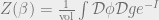
Gravity is a difficult concept to understand as a quantum theory. Therefore physicists (and their mathematician friends) study quantum gravity in 2 dimensions where equations are more tractable. Just like any good quantum theory, the path integral for quantum gravity is defined by where “vol” is the volume of the diffeomorphism group implying that the integration should be done on and upto diffeomorphism and is the action of a model knowns as Jackiw-Titelboim (JT) theory. Once the partition function is known, a quantum theory can be solved.
The partition function for the 2 dimensional quantum gravity (after imposing appropriate boundary conditions on two manifold with the topology of a disc) turns out to be where . is the renormalized coefficient for Einstein-Hilbert term (ignore it if you don’t know what it means).
Holographic duality
From AdS/CFT correspondence we know that the 2 dimensional quantum gravity is dual to 1 dimensional simple quantum system on the boundary of . This implies that the partition function that we computed earlier form JT model should be where is the Hamiltonian operator of the associated 1 dimensional quantum system. In other words, . This clearly is not equal to the partition function computed in the previous paragraph and that is problematic. The dual theories should have same partition function
Random Matrix theory
The idea here is to consider an ensemble of random matrices (with certain properties) and define the ensemble average of the partition function . In the matrix literature it is common to work with the inverse Laplace transform of the partition function given by known as the resolvent. So the resolvent correlation function has the “genus” expansion as follows (it is asymptotic series expansion) where is the dimension of the matrices of the ensemble. The terms can be computed systematically from what are known as “loop equations”, in terms of which is the “average density of the eigenvalues of random matrix of the ensemble”. The loop equations are streamlined into simple recursion relations which yield the correlation function upto all orders (in ) once is specified.
2 dimensional gravity again
In the JT model, there is a prescription to compute the quantity which involves integrating over connected 2d geometries with specified boundary length and value of dilation field at the boundary. The partition function turns out to be where is the length of a geodesic and is the Weil-Petersson volume of moduli space of Riemann surface with genus .
In the phenomenal paper Maryam Mirzakhani showed that the Weil-Petersson volume follow certain recursion relation which was shown to be equivalent to the recursion relation of matrix ensemble, we saw earlier, if we use the leading (genus 0) contribution of the JT path integral as thus resolving the problem described earlier.
There is analogous story for supersymmetric quantum gravity but I am in no mood to write about it. If you are interested read this paper by Witten and Stanford.


 where “vol” is the volume of the diffeomorphism group implying that the integration should be done on
  and
and  upto diffeomorphism and
  is the action of a model knowns as
  with the topology of a disc) turns out to be
  where
where  .
.  is the renormalized coefficient for Einstein-Hilbert term (ignore it if you don’t know what it means).
 where
where  is the Hamiltonian operator of the associated 1 dimensional quantum system. In other words,
  . This clearly is not equal to the partition function computed in the previous paragraph and that is problematic. The dual theories should have same partition function
 . In the matrix literature it is common to work with the inverse Laplace transform of the partition function given by
 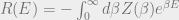 known as the resolvent. So the resolvent correlation function has the “genus” expansion as follows
  (it is
  is the dimension of the matrices of the ensemble. The terms
  can be computed systematically from what are known as “loop equations”, in terms of
  which is the “average density of the eigenvalues of random matrix of the ensemble”. The loop equations are streamlined into simple recursion relations which yield the correlation function upto all orders (in
  ) once
  which involves integrating over connected 2d geometries with specified boundary length and value of dilation field at the boundary. The partition function turns out to be
  where
where  is the length of a geodesic and
  is the Weil-Petersson volume of moduli space of Riemann surface with genus