Posted by

Posted on

July 23, 2019

Posted under

Comments

B for Behavior, Blackboard and Brain (2)

This post is continuation of this blog-post. Here we will understand the algorithm behind the emergent behavior, called Reinforcement Learning (RL). The situation of shooting colored boxes is equivalent to k-armed bandit problem which can be stated as

You are faced repeatedly with a choice among k different options, or actions. After each choice you receive a numerical reward chosen from a stationary probability distribution that depends on the action you selected. Your objective is to maximize the expected total reward over some time period, for example, over 1000 action selections, or time steps.

The reward for this game is: 100 for shooting red box and -10 for shooting blue box. The AI agent can access the scoreboard and take the actions accordingly. Based on the rewards, the agent generates the expected value associated to an action. This value is, in a way, the memory of all the rewards obtained when that particular action was performed. In more complicated systems, the rewards my be even probability based.

For RL, it is not only important to take those actions which have high expected value associated with them (exploiting the knowledge-base), but, once in a while, it is necessary to pick a random action irrespective of the associated expected value (exploration). This makes sure that the system doesn’t get stuck in the local optimum. For instance in case of correlated rewards, some actions when performed in certain sequence might yield better rewards. Later in this post it is shown why exploring leads to global optimum configuration knowledge!

For the problem at hand, the rewards are deterministic and static. So the RL algorithm is as follows (this algorithm can be found in Sutton’s book, section 2.4 (working link July 23, 2019))

Initialize, for $a = 1$ to $k$ :
$Q(a) \leftarrow 0$
$N (a) \leftarrow 0$
Repeat forever:

$\text{arg } \text{max}_a Q(a)$ with probability $1-\epsilon$ or a random action with probability $\epsilon$

$R \leftarrow \text{bandit}(A)$
$N (A) \leftarrow N (A) + 1$
$Q(A)\leftarrow Q(A) + \frac{1}{N(A)}\left[R - Q(A)\right]$

In Unreal Engine, the above algorithm can be easily implemented and is posted here (specifically look the member function UMAIBrainComponent::TickComponent). The game is played in the Unreal Editor where the rendered arena image is

Arena

The first two red boxes on left are levers 0 and 1 and last two boxes on right are 3 and 2 levers.

When the game begins, the control is passed over to AI agent who, as per the logic flowing through Tick function, starts shooting the boxes implementing RL technique. The log of first 22 iterations of the shootouts performed on July 23, 2019 can be found here.

Log Analysis:

We start with 0th iteration. An action (lever) is chosen at random because all the estimates are set to 0. The reward obtained is 100 and the estimate of action 0 is updated. For the next 3 iterations, the action with the highest expected value is chosen by the agent which results in pawn firing at first red box. But during 5th (marked with iteration number 4) iteration, the agent explores and randomly* chooses action 2 (last blue box) in spite of its expected value as 0. As result reward is -10. But then again it starts exploiting the knowledge-base and obtains higher rewards. Then again during iteration number 11 it chooses action 3 (second last blue box) and gets negative reward. Again, it continues with highest reward action selection (based on knowledge-base).

Finally during iteration number 19, it chooses action 1 (second red box) and gets reward 100. The estimates are updated (as can be see from next iteration’s maximum estimates ) and now, agent has global high estimates in the knowledge-base which couldn’t have been registered if agent weren’t exploring.

In the next blog-post of this series, we will see the visual implementation of this logic (natural to UE codebase).

* Ignore the 1 – epsilon text typo in the log text.

Posted by

ravimohan

Posted on

July 20, 2019

Posted under

The holographic view

Comments

2 Comments

B for Behavior, Blackboard and Brain (1)

Blackboard is a very efficient tool utilized by AI agent for generating appropriate behavior. In this blog-post I shall demonstrate the Unreal Engine code, in action, using the BlackBoard class.

First we initialize the BlackBoard object in the following fashion with line 8


void AMAIController::SetGameRep(AMAIGameState *GR)
{
MAIGameRep = GR;

// setup blackboard component
if(!MAIGameRep->GetBlackBoard())
{
UBlackboardComponent* BB = NewObject(this, TEXT("BlackboardComponent"));
if(BB)
{
BB->RegisterComponent();
MAIGameRep->SetBlackBoard(BB);

UBlackboardData* BlackboardAsset = NewObject(BB);
BlackboardAsset->UpdatePersistentKey(FName("PlayerScore"));
BB->InitializeBlackboard(*BlackboardAsset);
}
}

}

Then, we register the component with line 11 and declare the UBlackBoardData with line 14. Next we add the key PlayerScore in the UBlackBoardData and finally initialize the BlackBoard with the asset. This is the code equivalent to the editor state shown below

bbeq

The BlackBoard keys can be accessed by the code


GetGameRep()->GetBlackBoard()->GetValueAsFloat(FName("PlayerScore"));

The idea behind the BlackBoard is to provide a scratch work space with relevant data, required for the decision making purposes. Furthermore it is equipped with the ability to send notifications once data has been updated and cache the calculations saving redundant CPU processing time and power.

BlackBoard can be shared among several AI instances. It basically provides a common ground for all the AI instances to operate in collaborative manner. This gives rise to new collective behavior leading to more realistic gameplay and recreation.

Next, we want to focus our attention towards Reinforcement Learning algorithms which are more or less dormant in the game AI world (I really don’t have the clue why). But good news is that people are now gearing towards its implementation in game Engines (Unity seems first one to include that). For more information watch this video. There have been some white papers based on RL in game AI for instance Capture The Flag: the emergence of complex cooperative agents and Implementing Reinforcement Learning in Unreal Engine 4 with Blueprints.

Using the BlackBoard class, I applied Reinforcement Learning on Unreal Engine AI controller which is shown in the video below

The aim was to train the AI to shoot red boxes without actually coding it. This is called emergent behavior which was not included in the compiled code, but based on the rewards, AI learnt to shoot red boxes! More information on how I implemented RL will follow in the sequel blog-post. Stay tuned.

Posted by

ravimohan

Posted on

July 18, 2019

Posted under

The holographic view

Comments

Behavior Trees in Game Artificial Intelligence

Due to circumstances beyond my present control, my career trajectory has taken a sharp turn (quantified by delta function ). I hope Dirac would be proud of that! In order to work with same passion and rigor, I have channelized my energy into Artificial Intelligence (AI) and parted ways from Physics. Of course it was painful and depressing, but I found that even such feelings have utility in the catharsis. This blog-post is an attempt to show just that!

The gaming industry has played pivotal role in reshaping the modern networking architecture and graphics rendering (replication, realistic rendering and ray tracing). Therefore it is not unreal to expect the industry to push forward the AI realm. This can be estimated from sheer number of players in games like Fortnite (250 million), Halo and GTA V among others. Any breakthrough in the field of AI can be conveniently and collectively scrutinized by millions of players, facilitated by streamline workflow including developers, players and academics.

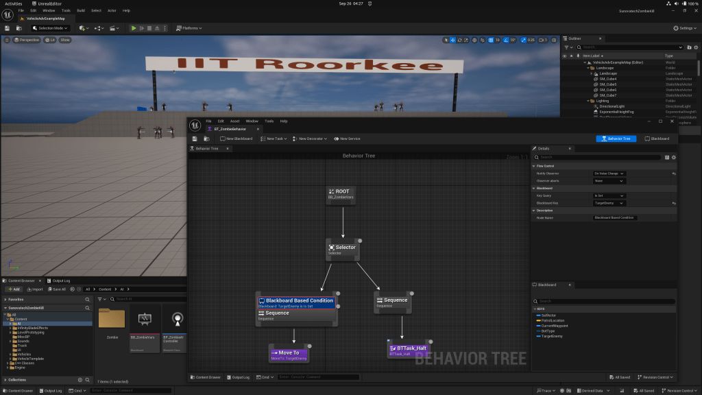
Behavior tree (BT) is an important mathematical structure which generates appropriate series of tasks in modular fashion. For instance, a patrolling pawn in some evil fortress. Unreal Engine (UE) is one of the very first game engines to implement BT in very natural way (given the visual scripting structure of UE called Blueprints). I will demonstrate the BT in action using UE project in this blog-post.

The BT can be pictured as

behaviortree

Here black nodes represent the “composites” (from of flow control) and pink nodes represent “tasks”. I have used two categories of composites

Selector: Executed in left-right pattern. It stops traversing the subtrees once successful execution branch is found.
Sequence: Executed in left-right pattern. It doesn’t stop executing subtrees until unsuccessful execution branch is found.

The entire BT is executed top-down pattern in deterministic way. A next level implementation could involve assigning probabilities with each edge resulting in particular node, but we won’t talk about that here.

If you were to petrol, what would be the list of tasks you’d make to execute. Probably it might include

Spotting enemy
Chasing enemy if spotted
Else perform random patrol in arbitrary directions

Now next step is to further divide the tasks into single elemental entities. For instance spotting enemy task includes checking lineofsight actors and spin towards appropriate actor if found. Thus the hierarchy and placement of composites and task should be as shown in the figure above.

Now BT in action corresponding to the chase is shown below.

Chase

One can clearly visualize the train of executing branches of the tree. Since Chase Player is a sequence node, we can deduce that the tasks “Rotate to face BB entry” and “BTT_ChasePlayer” have been executed and now “Move To” task is undergoing and indeed that is what is being done in the Editor.

Next, the BT simulation of patrolling with that task “Move To” is

petrol_moveto

and “Wait” is

petrol_wait

The complete information to setup the project is detailed at https://docs.unrealengine.com/en-US/Engine/ArtificialIntelligence/BehaviorTrees/BehaviorTreeQuickStart/index.html. I encourage to try!

Finally I will give a teaser to upcoming UE project https://github.com/ravimohan1991/MAI

Posted by

ravimohan

Posted on

August 5, 2017

Posted under

The holographic view

Comments

On-shell bosonic supersymmetric brane configuration

800px-calabi-yau

It has been, again, a long time, since I last wrote my blog-post! It is not that I don’t want to write, it is just that I have been having so much fun (doing my research) and somewhat busy (changing my apartment and doing similar non-productive chores). Now that I am within fewer steps away from my department, and that I have decided to spend rest of my PhD days in this new apartment, I can devote more time to writing.

This post is about kappa symmetry which is a tool to obtain the supersymmetric brane configurations. Now, Susy (the heart of my research), is not only the most beautiful and difficult 😉 symmetry but also the strongest symmetry that I have ever encountered. For some theories, it turns out that a supersymmetric configuration automatically implies the equations of motion (the on-shell configuration)! Therefore, supersymmetric theories without the Lagrangian formalism can be probed and studied! Furthermore, there are usually alluring geometrical interpretations associated with the configurations.

Currently I am working out the solutions of some supersymmetric brane embeddings on a curved supergravity spacetime geometry (with the topology $AdS_5\times\mathcal{C}\leftarrow S^1\times S^2\times S^1$ ), which, according to the AdS/CFT correspondence, represent line defects (analog of Wilson & t’Hooft lines) in the mysterious (2,0) super-conformal field theories in $d=6$ .

Consider any SUGRA with bosonic ( $\mathcal{B}$ ) and fermionic ( $\mathcal{F}$ ) degrees of freedom. Now it turns out that one can set the $\mathcal{F}=0$ on-shell. I don’t clearly see that, but it seems that the supersymmetry constraints the theory to that extent that equations of motion render the $\mathcal{F}$ non-dynamical! This also means setting $\mathcal{F}=0$ implies equations of motion. Now the question whether the $\mathcal{B}$ configuration preserves supersymmetry reduces to the question that what transformation parameters $\epsilon$ exist for on-shell bosonic configurations. Symbolically, $\delta\mathcal{B}|_{\mathcal{F}=0}=0$ while $\delta\mathcal{F}|_{\mathcal{F}=0}=0$ . The structure of local supersymmetry in SUGRA is given by $\delta\mathcal{B}\propto\mathcal{F}$ and $\delta\mathcal{F}\propto\mathcal{P}(\mathcal{B})\epsilon$ . Here $\mathcal{P}$ is a Clifford valued operator with maximum first order derivatives.

The previous statements imply $\mathcal{P}(\mathcal{B})\epsilon = 0$ . Now we note couple of points

The equation constraints the $\mathcal{B}$ degrees of freedom via first order (in some cases I know, linear) partial differential equations which are much simpler than the second order on-shell differential equations. Thus the complexity is greatly reduced!
The equation also constraints the transformation parameter $\epsilon$ in accordance with the bosonic configuration. For SUGRA geometry, we have what are known as Killing spinors which are solution of Killing equations corresponding to the bosonic degrees of freedom known as metric. For example, $d=11$ , $\mathcal{N}=1$ supergravity, $\mathcal{F}$ consists of gravitini $\Psi_a$ , the supersymmetric partner of graviton (the metric). Then $\delta\Psi_a=\left(\partial_a+\frac{1}{4}\omega_a^{bc}\Gamma_{bc}\right)\epsilon-\frac{1}{288}\left(\Gamma_a^{bcde}-8\delta_a^b\Gamma^{cde}\right)R_{bcde}\epsilon$ $= \mathcal{P}(\mathcal{B})\epsilon$ . Thus the equation $\delta\Psi_a=0$ gives the solution of Killing spinor.

As of now, we don’t have the complete formulation of M-theory (a unification of five superstring theories). We have a good idea of how M-theory should look like at low energies. In other words, we know the dynamical degrees of freedom with large wavelengths and they make up supergravity theory (that we know and understand) + M branes. We even have a Lagrangian for the theory at that energy scale which is given by

$S\approx S_{SUGRA} + S_{\text{Brane}}$

The first term corresponds to $\mathcal{N}=2$ $d=10$ type II A/II B supergravity or $\mathcal{N}=1$ $d=11$ supergravity. The second term describes both the brane excitations (giving rise to field theories) and interactions with the gravity. The action here is known as brane effective action.

Now for my research purpose, I am supposed to find the placement of M2 brane in the SUGRA background (mentioned above) such that there is a supersymmetric bosonic configuration. The placement of brane is based on $\mathcal{B}$ . Here again we set the $\mathcal{F}=\theta=0$ which is compatible with the on-shell configuration (brane equation of motion). To get the supersymmetric configuration

$\delta\theta=\delta_\kappa\theta+\epsilon+\Delta\theta+\xi^\mu\partial_\mu\theta=0$

where

$\delta_\kappa\theta$ is the kappa symmetry
$\xi^\mu\partial_\mu\theta$ world volume diffeomorphism
$\Delta\theta$ is any other transformation besides supersymmetry generated by $\epsilon$ .

Now again due to the reasons beyond me for now, the restriction of these transformations for the bosonic configuration

$\delta_\kappa\theta|_{\mathcal{B}}=(1+\Gamma_\kappa|_\mathcal{B})\kappa$
$\Delta\theta|_\mathcal{B}=0$ (makes sense since transformations by $\epsilon$ are fermionic!)

Hence

$\delta\theta=(1+\Gamma_\kappa|_\mathcal{B})\kappa+\epsilon$

Now it turns out that not all the fermionic degrees of freedom in this theory are dynamical. This forces us to work at the intersection of kappa symmetry gauge fixing conditions and $\theta=0$ . So we follow a two step process

Kappa symmetry invariance: $\mathcal{P}\theta=0$ where $\mathcal{P}$ is field independent gauge fixing projector such that $\theta = \mathcal{P}\theta+(1-\mathcal{P})\theta$ . And now the restriction of supersymmetric variation to bosonic configuration is
$\delta\mathcal{P}\theta|_{\mathcal{B}}=\mathcal{P}(1+\Gamma_{\kappa}|_\mathcal{B})_\kappa+\mathcal{P}\epsilon$ Equating this to 0 gives $\kappa = \kappa(\epsilon)$ the compensating kappa transformation corresponding to the background spinor.
Now we have the dynamical set of fermionic configuration given by $(1-\mathcal{P})\theta|_{\mathcal{B}}$ which we set to 0.

Now from the above equations and little bit of linear algebra, we finally have $\Gamma_\kappa|_\mathcal{B}\epsilon=\epsilon$ which is known as the kappa symmetry constraint.

Posted by

ravimohan

Posted on

February 20, 2017

Posted under

Uncategorized

Comments

Geometrical representation of the Killing spinors preserving N=4 supersymmetry (I)

In the low energy limit the mysterious M-theory boils down to a much tractable d=11 Supergravity theory (SUGRA). Therefore it is essential to understand the supersymmetric constraints of the theory which have crucial applications in the field of holography.

Supersymmetry is essentially a (very awesome if you ask me!) symmetry which keeps the theory invariant under the bosonic and fermionic variations given by

$\delta_\epsilon\Theta =\epsilon\\\delta_\epsilon X^M=i\bar{\epsilon}\Gamma^M\Theta$

Here $\epsilon$ is a Killing spinor which satisfies the Killing equation

$\nabla_X\epsilon=\lambda X.\epsilon$

It becomes covariantly constant for $\lambda =0$ . In the curved solutions of the SUGRA, supersymmetries are broken due to the non trivial covariant derivative. In order to preserve SUSY, the solutions of the Killing equation play essential role. We focus on those spinors which are invariant under the spin lift of the holonomy group of the appropriate manifold. For d=11 SUGRA, the Killing equation takes the following algebraic form

$\nabla_M\epsilon+\frac{1}{288}\left(\Gamma_M^{NPQR}-8\delta^N_M\Gamma^{PQR}\right)G_{NPQR}\epsilon=0$

Now the notion of the G-structures essentially classifies the special differential forms which arise in the supersymmetric flux compactifications. As can be deduced from the Killing equation, the solutions characterize the Spin Bundle of the supersymmetries with the metric of the manifold with a spin structure in a very intimate way.

Definition: A spin structure on a manifold $(\mathcal{M},g)$ with signature $(s,t)$ is a principle $Spin(s,t)$ -bundle with $Spin(\mathcal{M})\to \mathcal{M}$ together with a bundle morphism $\phi : Spin(\mathcal{M})\to SO(\mathcal{M})$ .

To define the G-structure, we associate the differential forms with the Killing spinors as follows

$\Omega^{ij}_{\mu_1\mu_2\ldots\mu_k}=\bar{\epsilon}^i\Gamma_{\mu_1\mu_2\ldots\mu_k}\epsilon^j$

The aim is to show that these differential forms obey the set of the first order differential equations as a natural consequence of the Killing equations. Now it can be shown that for Clabi-Yau manifolds, or manifolds with the $G_2$ holonomy, one usually finds the Killing spinor bundles trivially defined by an algebraic projection which are some differential forms applied to the complete spin bundle.

So this seems like a good point to start and make an ansatz for the projection operator for the spin bundle structure in the curved spacetime. These projections are essentially the differential forms defined above which give rise to the notion of the $G_2$ structures.

Here (for the reasons beyond me right now), three projection operators are defined $\Pi_j$ for $j=0,1,2$ which break the 32 supersymmetries to four. Another factual data is that if there is a holographic dual to the theory with a Coulomb branch, then there is a non-trivial space of the moduli for brane probes. This moduli space will be realized as conformally Kahler section of the metric (for four supersymmetries). And it is on this section of the metric, supersymmetries will satisfy projection conditions $\Pi_j\epsilon=0$ with the form $\Pi_j=\frac{1}{2}(1+\Gamma^{\xi_j})$ , where $\Gamma^{\xi_j}$ represents the product of gamma matrices parallel to the moduli space of the branes.

Now we can find the equations of motion of the theory by demanding that the fermionic variations vanish, implying the Killing equation! The solution we are considering here essentially has the topology of $AdS_4\times S^7$ . Using the orthonormal frames, https://arxiv.org/pdf/hep-th/0403006.pdf shows the presence of a Kahler structure on the brane-probe moduli space as a conformal multiple of

$J_{\text{moduli}}=e^6\wedge e^9+e^7\wedge e^8-e^5\wedge e^{10}$

I will continue from here in the next blog-post!

Ravi Mohan

If you haven't found something strange during a day, it hasn't been much of a day. – J. A. Wheeler

B for Behavior, Blackboard and Brain (2)

Log Analysis:

B for Behavior, Blackboard and Brain (1)

Behavior Trees in Game Artificial Intelligence

On-shell bosonic supersymmetric brane configuration

Geometrical representation of the Killing spinors preserving N=4 supersymmetry (I)