05 | August | 2017 | Ravi Mohan

800px-calabi-yau

It has been, again, a long time, since I last wrote my blog-post! It is not that I don’t want to write, it is just that I have been having so much fun (doing my research) and somewhat busy (changing my apartment and doing similar non-productive chores). Now that I am within fewer steps away from my department, and that I have decided to spend rest of my PhD days in this new apartment, I can devote more time to writing.

This post is about kappa symmetry which is a tool to obtain the supersymmetric brane configurations. Now, Susy (the heart of my research), is not only the most beautiful and difficult 😉 symmetry but also the strongest symmetry that I have ever encountered. For some theories, it turns out that a supersymmetric configuration automatically implies the equations of motion (the on-shell configuration)! Therefore, supersymmetric theories without the Lagrangian formalism can be probed and studied! Furthermore, there are usually alluring geometrical interpretations associated with the configurations.

Currently I am working out the solutions of some supersymmetric brane embeddings on a curved supergravity spacetime geometry (with the topology $AdS_5\times\mathcal{C}\leftarrow S^1\times S^2\times S^1$ ), which, according to the AdS/CFT correspondence, represent line defects (analog of Wilson & t’Hooft lines) in the mysterious (2,0) super-conformal field theories in $d=6$ .

Consider any SUGRA with bosonic ( $\mathcal{B}$ ) and fermionic ( $\mathcal{F}$ ) degrees of freedom. Now it turns out that one can set the $\mathcal{F}=0$ on-shell. I don’t clearly see that, but it seems that the supersymmetry constraints the theory to that extent that equations of motion render the $\mathcal{F}$ non-dynamical! This also means setting $\mathcal{F}=0$ implies equations of motion. Now the question whether the $\mathcal{B}$ configuration preserves supersymmetry reduces to the question that what transformation parameters $\epsilon$ exist for on-shell bosonic configurations. Symbolically, $\delta\mathcal{B}|_{\mathcal{F}=0}=0$ while $\delta\mathcal{F}|_{\mathcal{F}=0}=0$ . The structure of local supersymmetry in SUGRA is given by $\delta\mathcal{B}\propto\mathcal{F}$ and $\delta\mathcal{F}\propto\mathcal{P}(\mathcal{B})\epsilon$ . Here $\mathcal{P}$ is a Clifford valued operator with maximum first order derivatives.

The previous statements imply $\mathcal{P}(\mathcal{B})\epsilon = 0$ . Now we note couple of points

The equation constraints the $\mathcal{B}$ degrees of freedom via first order (in some cases I know, linear) partial differential equations which are much simpler than the second order on-shell differential equations. Thus the complexity is greatly reduced!
The equation also constraints the transformation parameter $\epsilon$ in accordance with the bosonic configuration. For SUGRA geometry, we have what are known as Killing spinors which are solution of Killing equations corresponding to the bosonic degrees of freedom known as metric. For example, $d=11$ , $\mathcal{N}=1$ supergravity, $\mathcal{F}$ consists of gravitini $\Psi_a$ , the supersymmetric partner of graviton (the metric). Then $\delta\Psi_a=\left(\partial_a+\frac{1}{4}\omega_a^{bc}\Gamma_{bc}\right)\epsilon-\frac{1}{288}\left(\Gamma_a^{bcde}-8\delta_a^b\Gamma^{cde}\right)R_{bcde}\epsilon$ $= \mathcal{P}(\mathcal{B})\epsilon$ . Thus the equation $\delta\Psi_a=0$ gives the solution of Killing spinor.

As of now, we don’t have the complete formulation of M-theory (a unification of five superstring theories). We have a good idea of how M-theory should look like at low energies. In other words, we know the dynamical degrees of freedom with large wavelengths and they make up supergravity theory (that we know and understand) + M branes. We even have a Lagrangian for the theory at that energy scale which is given by

$S\approx S_{SUGRA} + S_{\text{Brane}}$

The first term corresponds to $\mathcal{N}=2$ $d=10$ type II A/II B supergravity or $\mathcal{N}=1$ $d=11$ supergravity. The second term describes both the brane excitations (giving rise to field theories) and interactions with the gravity. The action here is known as brane effective action.

Now for my research purpose, I am supposed to find the placement of M2 brane in the SUGRA background (mentioned above) such that there is a supersymmetric bosonic configuration. The placement of brane is based on $\mathcal{B}$ . Here again we set the $\mathcal{F}=\theta=0$ which is compatible with the on-shell configuration (brane equation of motion). To get the supersymmetric configuration

$\delta\theta=\delta_\kappa\theta+\epsilon+\Delta\theta+\xi^\mu\partial_\mu\theta=0$

where

$\delta_\kappa\theta$ is the kappa symmetry
$\xi^\mu\partial_\mu\theta$ world volume diffeomorphism
$\Delta\theta$ is any other transformation besides supersymmetry generated by $\epsilon$ .

Now again due to the reasons beyond me for now, the restriction of these transformations for the bosonic configuration

$\delta_\kappa\theta|_{\mathcal{B}}=(1+\Gamma_\kappa|_\mathcal{B})\kappa$
$\Delta\theta|_\mathcal{B}=0$ (makes sense since transformations by $\epsilon$ are fermionic!)

Hence

$\delta\theta=(1+\Gamma_\kappa|_\mathcal{B})\kappa+\epsilon$

Now it turns out that not all the fermionic degrees of freedom in this theory are dynamical. This forces us to work at the intersection of kappa symmetry gauge fixing conditions and $\theta=0$ . So we follow a two step process

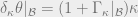
Kappa symmetry invariance: $\mathcal{P}\theta=0$ where $\mathcal{P}$ is field independent gauge fixing projector such that $\theta = \mathcal{P}\theta+(1-\mathcal{P})\theta$ . And now the restriction of supersymmetric variation to bosonic configuration is
$\delta\mathcal{P}\theta|_{\mathcal{B}}=\mathcal{P}(1+\Gamma_{\kappa}|_\mathcal{B})_\kappa+\mathcal{P}\epsilon$ Equating this to 0 gives $\kappa = \kappa(\epsilon)$ the compensating kappa transformation corresponding to the background spinor.
Now we have the dynamical set of fermionic configuration given by $(1-\mathcal{P})\theta|_{\mathcal{B}}$ which we set to 0.

Now from the above equations and little bit of linear algebra, we finally have $\Gamma_\kappa|_\mathcal{B}\epsilon=\epsilon$ which is known as the kappa symmetry constraint.

Ravi Mohan

If you haven't found something strange during a day, it hasn't been much of a day. – J. A. Wheeler

Daily Archives: August 5, 2017

On-shell bosonic supersymmetric brane configuration