All physical phenomena we see around us take place on something that we call spacetime. Therefore it becomes important to get acquainted with spacetime and understand how it affects the physical phenomena or gets affected by them. I will chronologically introduce the notions associated with spacetime because, usually, everyone gets to learn it in the exact same fashion.
Until 20th century, space and time were thought as different entities. It was thought that there exists a three dimensional euclidean space which acts as a stage for the physical phenomena. This stage was supposed to be rigid, static and flat (rigorous definition will be given later). The space was a three dimensional extension of Euclid’s five axioms for plane geometry which were
Between two points in the space, only one line can be drawn.
A finite line in a space can be extended indefinitely.
A circle with arbitrary radius and center can be drawn in the space
All right angles are equal to one another.
If a straight line falling on two straight lines make the interior angles on the same side less than two right angles, the two straight lines, if produced indefinitely, meet on that side on which are the angles less than the two right angles.
These axioms were based on the human experience (at the time of Euclid) and considered to be true in every part of the universe. Even now, based on high-school experience, one doesn’t need enough convincing about the validity of these postulates.
Let us now define our three-dimensional Euclidean space in formal way. It is a set of points with well defined distance between any two points of the set. If you give me two points say and belonging to Euclidean space. I will give you the distance between them by computing .
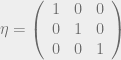
A couple of interesting points can be noted. First, the definition of distance between two points is static i.e the way to find distance doesn’t change with time. We can represent the definition of distance between two points using matrices. Let us represent the points by column matrices and and define a matrix . The distance between two points can now be given by (here ‘.’ represents matrix multiplication). Note that the definition of distance depends on the matrix . Physicists and mathematicians call metric of the space. Now we can say that it is the metric which defines the distance between two points of a space. In fact the metric defines the notion of a ‘dot product’ in a space. Take any vector, write its components in column matrix and used the matrix multiplication defined above to find the length of the vector.
The metric of Euclidean space is time independent (build from constant numbers). Although I have used matrix to represent a metric, generally it should be thought as a set of numbers given by where .
Next we note that the metric (of Euclidean space) is independent of space itself. In fact this independence is a direct consequence of Euclid’s axiom 5. This independence implies that the space is flat. I will demonstrate this and provide a formal definition of flatness in a later post.
Yes, I am aware of the ennui caused by this topic. We write schrodinger’s time independent equation, solve it, apply the boundary conditions, find the energy eigen states, normalize them and everybody is happy. If you are a physics major, then you must have done this countless times. But I always had a problem with this system because of its highly un-physical nature (I will come back to this later). That makes it a mathematical curiosity and if it is, then why not explore it to the full extent? Please note that in this post I will use rigorous mathematics and will define terms in proper mathematical language (I hope this post will serve as my notes for future reference). Here one can also appreciate the aesthetics of Linear Algebra.
The question I had been asking myself was, “Why do we always work in position representation? What is wrong in working in momentum representation (for this particular problem)?”. The curiosity to find the answers compelled me to plunge into the depths that are generally not touched and mentioned in physics literature.
The conventional Quantum Mechanics (for this problem) is performed on the Hilbert Space which I will denote with . Here (read L two) represents a functional space of square integrable functions and represents the range of parameter (position). I am interested in working with and want to obtain energy eigen states in terms of the wavefunction . I dont know the range of the parameter (momentum). I can’t take it as whole real line (because of the bounded nature of position). Parseval-Plancherel theorem in not applicable here. I must first find the nature of momentum operator. Then maybe its spectrum might give me the idea about the range of momentum.
Just like a function has a domain, the linear operator on Hilbert space has a domain. The formal definition of the operator is (this definition is for general Hilbert Spaces and not restricted to L two spaces)
An operator on the Hilbert space is a linear map : such that (where ).
represents the linear subspace of . This subspace is the domain of the operator. Strictly speaking, Hilbert space operator is the pair which is the specification of the operation with the domain on which the operation is defined. Now two operators are said to be equal if and only if
for all .
Let us consider position operator denoted by . The operation is defined as . But given the boundary conditions, the domain is defined as
and .
As mentioned earlier, the Quantum Mechanics is performed on the Hilbert Space of square integrable functions (denoted by ), we certainly would not want a mapping which blows up the square integrability. Hence it is important to put the restriction that the output be which translates into . So, in words, the domain of is the set of all the square integrable functions such that
they satisfy boundary conditions
the output of linear map should be finitely square integrable
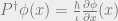
Now let us define momentum operator . Quantum Mechanics defines the operation of this operator (on a function) as
Certainly, we would like to have a set of those functions which besides satisfying boundary condition, also have square integrable derivatives. In formal language
and .
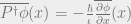
Now let us see the definition of the adjoint of an operator which means we have to define the operation and domain of the adjoint of operator (let’s denote it by ).
such that
This definition says that the domain of is set of (square integrable) such that there exists (again square integrable) which makes the equation true for all the belonging to domain of operator .
For a given , depends on and . The operation of is defined as
.
So we, now, have a full working definition of the adjoint of a operator. Let’s find the adjoint of . The inner product equation must hold. So
.
On integrating by parts, the RHS
.
For this equation to be true we must have
or
.
The most curious and interesting point is that the function does’t need to satisfy boundary condition (of infinite square well) since is zero as already satisfies the boundary condition. Clearly the has no restriction save square integrability which shows that the set has more elements than set . The formal definition of is
.
It can be seen that . Thus i.e the momentum operator is not self-adjoint. On the other hand it is quiet simple to show that i.e the position operator is self-adjoint.
Now let us see the definition of Hermitian operators.
The operator on is Hermitian if for all
Since operates on both the functions, needless to say, they must belong to the domain of the operator. Let us use the definition of adjoint operators. Operator is such that which implies . Thus if the operation of the operator is same as that of its adjoint, then it is Hermitian operator. The domain of both the operators need not be same.
We have seen that the specification of both and is same . The momentum operator is Hermitian for this case but not self-adjoint. It is easy to note that all the self-adjoint operators are Hermitian but vice-versa is not true.
Now the spectral theorem of linear operators states that
If the Hilbert space operator A is self-adjoint, then its spectrum is real and the eigenvectors associated to different eigenvalues are mutually orthogonal; moreover, the eigenvectors together with the generalized eigenvectors yield a complete system of (generalized) vectors of the Hilbert space.
This property does not hold for only Hermitian operators.
As the momentum operator, here, is only Hermitian its eigen vectors won’t form complete basis. Thus there is no use in solving this problem in momentum space. Moreover, space wont have continuous momentum (because of quantization imparted by boundary conditions).
Normally one assumes that the eigen vectors of an observable forms a complete set of basis. This means that observables must be represented by self-adjoint operators. From above we note that momentum operator is not an observable for this problem!
Absurd, isn’t it? Well, the boundary condition itself gives us the hint of the highly non-physical nature of the problem. The “non self-adjointness” of momentum operator further shows us how the infinite potential square well is a mathematical curiosity with tenuous nexus to real physical systems.
So it has been more than a week since I wrote my last blog post. Although, time to time, I was tempted to write the sequel, but I had to distance myself from that temptation. I have been studying David Griffiths’s “Introduction to Elementary Particles” and much of my time has been devoted to it. Hopefully one day I will know Particle Physics well enough to blog about it.
So by now I am sure you know what it means when we say something is linear. This is the beginning of linear algebra. It is a very beautifully constructed algebra which physicists use in their daily life (like in Quantum Mechanics, Special theory of Relativity and Classical Mechanics). I don’t intend to start off with the abstract Hilbert Spaces (basically a set of linear vectors with some axioms) and define linear maps, inner product structure and so on. Instead I will try to demonstrate the linear algebra “at work (using Quantum Mechanics)” without worrying too much about mathematical vigour. Now I must warn you that this mathematical vigour is absolutely necessary to not only appreciate the beauty of mathematics (I am a big fan of the water-tight derivations done by the mathematicians!) but to get a better understanding of Quantum Mechanics (least you land up in the situation where it might seem that Quantum Mechanics is inconsistent with itself). Basically in the following demonstration, I will define certain mathematical quantities in a very loose way (loose enough to drive any mathematician, with slightest respect for mathematics, crazy) and mix them with the postulates of Quantum Mechanics without explicitly stating them. For instance, the example I gave in last post, deals with the linear vectors belonging to a linear vector space equipped with inner product structure (or Hilbert Space). I believe that this way I wont make the subject abstract enough for the people new to Linear Algebra and Quantum Mechanics.
So Quantum Mechanics says that the physical states are linear. This might not surprise you and you might think that it is obvious (maybe after going through the example I gave in last post). But think again! This statement is powerful enough to lead to certain results which you might not consider obvious.
Before going further I want you to see this video and try to understand the problem it states in the end.
At first it might seem too confusing. But we will go, step by step, and try to reproduce the experimental results using Quantum Mechanics. I am considering the case when only one electron is shot out at a time from source . I associate a linear state vector to represent the electron at source. Now the states representing slit 1 and 2 be and respectively. The screen is basically a real number-line where each point represents a state written as . Note that is a continuous parameter here.
Now recall last post in which I gave an example of “creating” a set of persons “using” two persons (basis). In general a person can be written as where the will tell me the resemblance of person C with person A or B. Now I define a term inner product as a function (a linear map) which maps the ordered pair of linear vectors into a scalar complex number. This complex number gives the component of the linear vector on other linear vector ( will give resemblance).
Consider the inner product of person A and B written as . Now we know that they don’t resemble at all. Hence should be equal to (state B has no component on state A whatsoever). The states and are said to be orthogonal. Also we know that state completely resembles with itself and so does state . Thus (I can assign any number to this inner product). I have normalised the state vectors and (because the number I assigned is ). They are now called orthonormal linear vectors.
To find the component of along , I just need to evaluate the inner product . So
and
The resemblance of state C with state A is and with state B is . This is the idea of inner product.
In Quantum Mechanics it is used in a different way. We have state C (now representing a physical state and not a person) given in terms of state A and state B (again physical states). Now if a system is described by state then is the amplitude of state to exist in state (read it this way and understand it this way!). is the probability with which we will find a system described by state in state . The probability of state C to exist in state B is . So instead of resemblance, the component of vector gives an idea about the probability. This is the basic rule which the nature seems to follow. Max Born was the guy who realised this.
The question which might arise here is that before measuring the system it was in state . Mathematically it is called superposition of states and . But what is it physically? Does it mean that if a system is represented by state then it is existing in both the states and , simultaneously? Quantum Mechanics gives no answer to this. It is something that you have to interpret yourself.
Although you might try to relate it to the example I gave in previous blog post, but you must understand that these physical states are very different from the states representing the persons in the sense that there are no “extra variables” (like lefty, hindi and lazy) which make up the states. These states are fundamental and nothing is implicit. For instance state represents slit in double slit experiment and that is it. So from now on, the physical states are to be considered without any extra variables.
Now I define another linear entity “operator”. It is again a linear map (or function) which maps a linear vector into another linear vector. Operator is denoted by a letter with a hat . So the operation of a linear operator on a linear vector is defined as , where is a complex number. Now I can represent same operator by . This is known as “outer product notation”. Let’s check weather this notation is compatible with the definition of operator.
Here . State might not be normalised.
In Quantum Mechanics all kind of actions on a state vector are represented by linear operator. There are operators corresponding to time translation, space translation, space rotations and observables. By definition theses operators map a linear vector (physical state) to another linear vector (another physical state).
Suppose you are standing on the other side of slit (opposite to electron source). Further suppose that slit is closed. Now what state would you assign to the electrons coming out towards you? Now the slit will act like a source. You will say that the state of electron is . Thus the state has been mapped to state . This is the handiwork of slit and thus we should associate an operator with it. How should the operator look like? Operator should be able to tell us the amplitude of state to exist in state . Consider the form . Now . This operator maps the state to state and also provides the required amplitude. So good! Similarly, on closing slit , we will find that the operator corresponding to slit is . In hat notation, I assign operators and to slit and respectively.
Now we have necessary tools to work out the Quantum Mechanics of this experiment. The states for double slit experiment we have are and and the operators are and . Now if I shoot one electron after other, then (assuming no absorption by the slit wall) I should be able to get corresponding detection at certain state (on the screen). So one electron is emitted out from source and we detect one electron on screen. I should evaluate the amplitude of state to exist in state or the number . Then I can get the probability with which an electron will be detected at by evaluating .
We saw that the slits have the ability to map state to state or state and these are the only two alternatives. This should make us conclude that state is made up of state and with certain amplitude (which is nothing but probability for state S to exist in slit 1 or 2) for each of them in a linear way. Thus
and
with little re-arrangement
Feynman’s way
In Feynman’s lectures volume III, he obtains the last equation in a very beautiful and intuitive way. He first states two rules
when an event can occur in several alternative ways, the probability amplitude of the event is the sum of amplitudes of each alternative way considered separately (provided experiment is not capable of determining which alternative is actually taken). If the experiment is capable of determining, then the probabilities should be added.
and
if a particle goes through a route then the amplitude for that route can be written as a product of amplitude to go part way and amplitude to go rest of the way.
In our double slit, the particle can reach state by two ways (which can not be distinguish just by detecting the electron at the screen) thus the amplitudes must add
The experiment is going via superposition of two possible alternatives. Now using second rule we can say that (I have changed the order since it is better to read from right to left). Similarly and we end up with the same equation.
Now is a complex number and so is , but is a continuous variable which can take any value like and so on and for every we should have corresponding amplitude. It is better to represent by a function say . Same goes for . Thus
.
You can put and inside the functions. It won’t be a problem becase they are constant.
The probability to detect a particle on screen (at certain y) is . So now you see why we get interference pattern? The probability contains a cross term which precisely shows interference.
You see, how by associating linear vectors to physical systems (and using some additional assumptions) we found an astonishing result of interference. If you want you can watch the video again (keeping this treatment in mind). Now I am going to discuss the physical implications of this treatment.
First you might be wondering about the nature of electron. Is it particle? Or is it a wave? Well it is neither. Wave and particle are classical concepts which are often mixed with the name “wave particle duality” to describe quantum entities. I consider it as misleading specially for new people learning Quantum mechanics. You see in Quantum Mechanics we just say that it is a linear vector by which we mean that it is an entity that is linear in nature. There is absolutely no need to draw a picture of the electron in your mind (like a rigid ball or wavy curve or mixture of both).
Now since it is a linear vector it can exist in superposition of various states. So it is not necessary to imagine an electron going through a particular slit (when you are not observing the electrons at the slit). It is going through both the slits (if this is what you want to hear). And in Quantum Mechanics you will come across such examples many times.
In the video you have seen that interference pattern disappears when one tries to observe the slits through which electron goes. So the act of measurement destroys interference pattern. Of course we can show that using Quantum Mechanics, but it involves concept of Tensor Product or Direct Product of linear vectors, which is out of the scope of this article. Feynman, on the other hand shows (by following those two rules) how the measurement destroys interference without “explicitly” talking in terms of direct product. I dont want to repeat it, so I recommend Feynman Lectures Vol III chapter 3.
This is called Schrondinger’s equation and it is often used in Quantum Mechanics. To understand this equation one should understand the mathematics on which Quantum Mechanics is based.
Note appearing on both the sides of the equation. Mathematicians call it “linear vector”.
In mathematics linear vectors are recognised by the following property:
On adding two linear vectors the entity obtained is again a linear vector.
The mathematical examples of linear vectors are numbers, integers, matrices and solutions of linear differential equations (there are more, think!). You can see that if you add two entities belonging to a type (say integer), then you end up with same type of entity again (integer) and not some other entity (matrix or irrational numbers). On the other hand solutions of non-linear differential equations are not linear vectors. If you add two solutions, the resultant function will not satisfy the equation!
In Quantum Mechanics we use linear vectors to represent the state of a physical system at certain time ‘t’. In physics, state of a system means the information of the various variables (in form of numbers) related to a system. If I know these numbers, I know the physical system through and through. And if I know these numbers as function of time, I know the dynamics of the system. One natural question which may arise is
If we know these numbers as function of time then does it mean we know the future of that physical system?
According to Classical Physics answer is yes (in principle), but in Quantum Mechanics we can only estimate the odds, so the answer is no (even in principle).
So Quantum Mechanics says that I can associate with any physical system (starting from electrons and molecules (even myself!) upto galaxy and beyond). All the information (set of numbers) associated with the physical system is buried inside this state vector. It is the job of physicist to extract the information and use it.
Quantum Mechanics is telling us that the properties of physical systems are linear in nature. If I add two physical states then the resulting state will also be a physical state!
Let us consider a physical example which explicitly shows this property of linear vectors. Then I will come back to explain what I said in last paragraph. Consider a city which is inhabited by only 8 people. Now each person has different characteristics which make him/her unique. For simplicity, let us consider that they have only three characteristics with two possible choices.
The hand they use to do work (lefty/righty)
The language they know (hindi/english)
Habit (lazy/active)
Let us consider a person ‘A’ having three characteristics as
Righty
Hindi
Active
and denote this person with linear vector . In the city if we search for set of characteristics mentioned above, it means we are searching for person A and thus we should use for these set of characteristics which describes the state.
Similarly, let there be person ‘B’ having characteristics
Lefty
English
Lazy
and denote this set or state with . Analyse the table and take its snapshot in your mind.
Person A or
Person B or
Phase ()
Work
Righty
Lefty
Language
Hindi
English
Habit
Active
Lazy
Now my aim is to show that one can represent other 6 persons using these two persons or in other words I can represent 6 other states using these two states ( and ). For the given scenario, the only possible way is to choose one characteristic from any one person and rest two from other. This way we can build 6 other set of characteristics (6 more states and hence 6 more people). Now we set the coefficients of and as the square root of number of characteristics picked from that particular state (I will explain the reason little later).
Consider a case: Select 1 characteristic of person A, say work, and rest from characteristics of person B, language and habit. The state thus formed is {Righty, English and Lazy} which neither represents person A nor person B. It represents new state or a new person denoted by . Here coefficient of denotes the square root of number of characteristics picked from person A and similarly coefficient of denotes the square root of number of characteristics picked from person B. I have divided whole linear vector by in order to normalize it. We can represent new person in terms of two special persons (call them basis).
Let us pause here and think why linear vectors are suitable to describe persons. We defined a person with a set of characteristics. And we know that if we add characteristics (in any proportion) we get another set of characteristics which describes another person (and not some animal!). This idea is important and this is what allowed us to use linear vectors for persons.
If you are wondering why I chose to take the square root of number of characteristics picked as coefficients, then now is the time to explain. We can say that the shows us the similarity to the person (or state) it is written with. Thus person C is 1/3 like person A and 2/3 like person B. Also it is obvious by the choices I made.
But this is not a correct way and there is a fallacy. If I select language of person A and rest two characteristic from person B then the state I get is {Lefty, Hindi and Lazy} which represents different person altogether (who is certainly not person C). So let us call him person D (if you did think this on your own then you are really paying attention). Hence I need one more variable to store one more piece of information. The information being what kind of choice is made first. The previously mentioned coefficients will tell me how many characteristics were picked from person A and B. So I need to concentrate on the person from which only one characteristic was chosen (because this choice will determine other two choices from other person). Hence I have introduced a term (call it phase) . Take a look in the table. The fourth column shows the phase associated with each characteristic (later I will explain the reason for this particular allotment of phase).
If I define the linear vector associated with person C as and person D as then everything will fall in right place. Not only I can see the mathematical difference between person C and D, but I am also able to preserve the definition of “likeliness” in the way that both the person C and D are 1/3 like person A and 2/3 like person B and still they are different!
No you might ask why did I assign phase like this. I considered the number of ways in which one characteristic is chosen from one person and two from another (for this case it is 3). I, then, divided by that number and allotted the phases accordingly.
Another question might rise at this point. What if we have a set of more than three characteristics? Will this method work? Certainly, the answer is yes. In that case you can consider all sorts of permutation and assign a phase to each permutation like I did in this case.
But why to divide the number ? Well it clearly means that I want to divide a circle in parts. The number of parts being equal to number of permutations calculated. Also I know that coefficients should vary from 0 to 1. So I can use sine and cosine of a parameter instead of these coefficients. Let that parameter be where varies from to . And we also know that the phase is varying from to (in parts). What do you make out of it? Have you seen these limits elsewhere? Yes, of course, these are the polar and azimuthal angles of a spherical-polar coordinate system where the length (defined as ) is constant as and are varied. The surface traced this way will be, no doubt, a sphere. Discreet points on the sphere represent the states (decided by the and of that point).
In general state representing a person can be written as
This sphere has special name Bloch’s Sphere. The only difference is that on our sphere we have discrete points where as on bloch sphere there are uncountable points and, hence, uncountably infinite states. and vary continuously.
Let us stop here conclude this post with following statements:
Anything (mathematical or physical) that is linear can be represented by linear vectors.
Quantum Mechanics says that all the physical systems are linear.
To represent the set of linear entities (in this example we had a set of 8 persons) we can find a subset of those entities (persons A and B), known as basis, to represent all the other entities.
In next post I will demonstrate how linear vectors are used in Quantum Mechanics.


![L^2 ([0,1], dx)](https://s0.wp.com/latex.php?latex=L%5E2+%28%5B0%2C1%5D%2C+dx%29&bg=eeeeee&fg=666666&s=0&c=20201002) which I will denote with
which I will denote with  . Here
  (read L two) represents a functional space of square integrable functions and
 ![[0,1]](https://s0.wp.com/latex.php?latex=%5B0%2C1%5D&bg=eeeeee&fg=666666&s=0&c=20201002) represents the range of parameter
represents the range of parameter  (position). I am interested in working with
  and want to obtain energy eigen states in terms of the wavefunction
  . I dont know the range of the parameter
  (momentum). I can’t take it as whole real line (because of the bounded nature of position). Parseval-Plancherel theorem in not applicable here. I must first find the nature of momentum operator. Then maybe its spectrum might give me the idea about the range of momentum.
 :
:  such that
  (where
  ).
). represents the linear subspace of
  which is the specification of the operation with the domain on which the operation is defined. Now two operators are said to be equal if and only if
 for all
  .
. . The operation is defined as
  . But given the boundary conditions, the domain is defined as
 and
and  .
. which translates into
 . So, in words, the domain of
  . Quantum Mechanics defines the operation of this operator (on a function) as
 and
and  ).
). such that
 is set of
  (square integrable) such that there exists
  (again square integrable) which makes the equation
  true for all the
  belonging to domain of operator
  ,
,  depends on
  .
. must hold. So
 .
.![\int_{0}^{1} \overline{P^{\dagger}\phi}(x) \psi (x) dx = \frac{\hbar}{\iota}\left[_{0}^{1} \overline{\phi}(x) \psi (x)\right] -\frac{\hbar}{\iota} \int_{0}^{1}\overline{\frac{\partial \phi}{\partial x}}(x) \psi (x) dx](https://s0.wp.com/latex.php?latex=%5Cint_%7B0%7D%5E%7B1%7D+%5Coverline%7BP%5E%7B%5Cdagger%7D%5Cphi%7D%28x%29+%5Cpsi+%28x%29+dx+%3D+%5Cfrac%7B%5Chbar%7D%7B%5Ciota%7D%5Cleft%5B_%7B0%7D%5E%7B1%7D+%5Coverline%7B%5Cphi%7D%28x%29+%5Cpsi+%28x%29%5Cright%5D+-%5Cfrac%7B%5Chbar%7D%7B%5Ciota%7D+%5Cint_%7B0%7D%5E%7B1%7D%5Coverline%7B%5Cfrac%7B%5Cpartial+%5Cphi%7D%7B%5Cpartial+x%7D%7D%28x%29+%5Cpsi+%28x%29+dx&bg=eeeeee&fg=666666&s=0&c=20201002) .
.
 .
. does’t need to satisfy boundary condition (of infinite square well) since
 ![\left[_{0}^{1} \overline{\phi}(x) \psi (x)\right] = \left[ \overline{\phi}(1) \psi (1) - \overline{\phi}(0) \psi (0) \right]](https://s0.wp.com/latex.php?latex=%5Cleft%5B_%7B0%7D%5E%7B1%7D+%5Coverline%7B%5Cphi%7D%28x%29+%5Cpsi+%28x%29%5Cright%5D+%3D+%5Cleft%5B+%5Coverline%7B%5Cphi%7D%281%29+%5Cpsi+%281%29+-+%5Coverline%7B%5Cphi%7D%280%29+%5Cpsi+%280%29+%5Cright%5D+&bg=eeeeee&fg=666666&s=0&c=20201002) is zero as
is zero as  already satisfies the boundary condition. Clearly the
  has more elements than set
  . The formal definition of
  .
. . Thus
  i.e the momentum operator is not self-adjoint. On the other hand it is quiet simple to show that
  i.e the position operator is self-adjoint.
 for all
 is such that
  which implies
  . Thus if the operation of the operator is same as that of its adjoint, then it is Hermitian operator. The domain of both the operators need not be same.
 is same
  . The momentum operator is Hermitian for this case but not self-adjoint. It is easy to note that all the self-adjoint operators are Hermitian but vice-versa is not true.
 . I associate a linear state vector
  to represent the electron at source. Now the states representing slit 1 and 2 be
  and
and  respectively. The screen is basically a real number-line where each point represents a state written as
  . Note that
  is a continuous parameter here.
 where the
  will tell me the resemblance of person C with person A or B. Now I define a term inner product as a function (a linear map) which maps the ordered pair of linear vectors into a scalar complex number. This complex number gives the component of the linear vector on other linear vector (
 will give resemblance).
 . Now we know that they don’t resemble at all. Hence
  should be equal to
  (state B has no component on state A whatsoever). The states
  and
and  are said to be orthogonal. Also we know that state
  (I can assign any number to this inner product). I have normalised the state vectors
  ). They are now called orthonormal linear vectors.
 along
along  . So
. So
 and
and 
 and with state B is
  . This is the idea of inner product.
 represents slit
  . So the operation of a linear operator on a linear vector is defined as
  , where
  is a complex number. Now I can represent same operator
  . This is known as “outer product notation”. Let’s check weather this notation is compatible with the definition of operator.
 . State
  might not be normalised.
 is closed. Now what state would you assign to the electrons coming out towards you? Now the slit
  . Now
. Now  . This operator maps the state
  . In hat notation, I assign operators
  and
and  to slit
  and
and  . Then I can get the probability with which an electron will be detected at
  .
.


 (I have changed the order since it is better to read from right to left). Similarly
  and we end up with the same equation.
 is a complex number and so is
  , but
, but  and so on and for every
  . Same goes for
  . Thus

 .
. and
and  inside the functions. It won’t be a problem becase they are constant.
 . So now you see why we get interference pattern? The probability contains a cross term which precisely shows interference.
 appearing on both the sides of the equation. Mathematicians call it “linear vector”.
 )
)

 . Here coefficient of
  in order to normalize it. We can represent new person in terms of two special persons (call them basis).
 . Take a look in the table. The fourth column shows the phase associated with each characteristic (later I will explain the reason for this particular allotment of phase).
 and person D as
  then everything will fall in right place. Not only I can see the mathematical difference between person C and D, but I am also able to preserve the definition of “likeliness” in the way that both the person C and D are 1/3 like person A and 2/3 like person B and still they are different!
 by that number and allotted the phases accordingly.
 ? Well it clearly means that I want to divide a circle in parts. The number of parts being equal to number of permutations calculated. Also I know that coefficients should vary from 0 to 1. So I can use sine and cosine of a parameter instead of these coefficients. Let that parameter be
  where
where  varies from
  . And we also know that the phase
  is varying from
  ) is constant as
  representing a person can be written as
